Blog
This article was contributed by Xinghong Fu, a Global Intern of Qfin team.
Introduction
Predicting the market is hard. There has been countless research in this direction, with various types of models being developed, including autoregressive (Box 1970), moving averages (McKenzie 1984), global univariate models like N-BEATS (Oreshkin et. al. 2020), and long-term forecasting models (Nie et. al. 2022). Following the work (Devlin et. al. 2019, Brown et. al. 2023) of large language models (LLMs) have also attempted to directly make use of LLMs zero-shot forecasting capabilities (Gruver et. al. 2023).
To our immediate interest is TimesFM (Das et. al. 2024), a recent work by Google in training a 200M parameter model for time series forecasting purposes. TimesFM has shown state-of-the-art (SOTA) performance on multiple benchmarks like Monash (Godahewa et. al. 2021), Darts (Herzen 2022) and ETT (Zhou 2021). However, also as with previous SOTA models in time series forecasting, these benchmarks include generic data such as weather, traffic and search trends, to name a few. Data such as these show regular patterns on daily, weekly or monthly scales that the model can capture these seasonalities to give accurate predictions.
However, financial data, in particular stock price data, is extremely irregular, barely showing any recognizable patterns and has a very low signal-to-noise ratio. So, it is unclear whether TimesFM can predict such an irregular time-series or not.
In this study, we aim to fine-tune TimesFM such that it can also give reliable forecasts in financial markets. Shown in figure 1, fine-tuning TimesFM can give significant improvements to its price prediction accuracy.
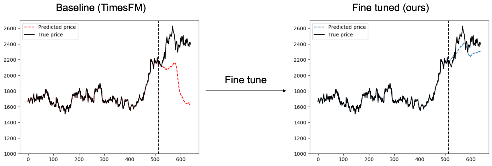
Figure 1: Fine tuning on financial data improves price prediction accuracy from the baseline TimesFM model
Fine-tuning on financial data
This section is a brief description on the data we used for fine-tuning and the fine tuning techniques and settings to continue the pre-training of TimesFM.
Data collection and description
We fine-tune TimesFM for the task of price prediction. Data is obtained from various sources, including historical price data for stocks listed in TOPIX500, S&P500, to name a few. More details can be found in Table 2.
| Dataset | Granularity | # Times series | # Time Points |
| Topix500 stocks | Daily | 3513 | 2248320 |
| S&P500 stocks | Daily | 3173 | 2030720 |
| Currencies | Daily | 1092 | 698880 |
| Japan Investment Trusts | Daily | 6698 | 4286720 |
| Commodities | Daily | 29 | 18560 |
| Stock Indices | Daily | 216 | 138240 |
| Stock Indices | Hourly | 847 | 542080 |
| Stock prices | Hourly | 31756 | 20323840 |
| Cryptocurrencies | Daily | 1680 | 1075200 |
| Cryptocurrencies | Hourly | 79153 | 50657920 |
Table 2: Description of dataset used for fine tuning.
To avoid look-forward biases, our train-eval set is taken from data up till 31 Dec 2022, with a 75-25 split respectively, and the test set contains data from 1 Jan 2023 onwards.
Fine tuning technique and settings
We implement continual pre-training as the fine-tuning method on financial data. This is the direct method of restarting training from the final pre-trained weights of TimesFM to focus on the financial data we gathered. In the backpropagation step of fine-tuning, we apply gradient update on weights of each layer of TimesFM.
The first problem we observed directly applying this training scheme is overfitting. Problematically, the original TimesFM employs mean-squared-error (MSE) loss, which is biased towards stock prices with originally high values. Such scale bias causes the model to fixate on specific time series examples during training and result in deteriorating performance in the evaluation set due to the failure in generalization.
To resolve this, we attempted to compute the percentage MSE loss. But due to extreme financial events such as flash crashes, like that for Hikari Tsushin in year 200 and LUNA in year 2022, training instabilities resulting in NaN loss occur, because the percentage changes during crashes exceed 10000%.
A solution that worked for us was taking the logarithm of the input data before passing it to the model. Namely, we perform the following transformation to the data: \(y \leftarrow \log(y) \)
The transformed data is then passed through the model and we then compute MSE loss on the resulting output. At inference time, we invert the transformations to output consistent results.
It is worth noting that when the price change is small, this is approximately equal to percentage MSE loss, but suppresses overwhelmingly large values at large changes to avoid instabilities.
With the following training recipe, we are able to complete fine-tuning of TimesFM without any NaN loss within 1 hour on 8 V100 GPUs.
| Hyperparameter/Architecture | Setting |
| Optimizer | SGD |
| Training epochs | 5 (linear warmup), 95 (cosine decay) |
| Peak learning rate | 1e-4 |
| Momentum | 0.9 |
| Gradient clip (max norm) | 1.0 |
| Batch size | 1024 |
| Max context length | 512 |
| Min context length | 128 |
| Output length | 128 |
| Layers | 20 |
| Hidden dimensions | 1280 |
Table 3: Hyperparameter settings for fine tuning TimesFM on financial data.
For ease of training, we construct time series of length 640 = max_context_length + output_length. Time series are appended with their last value until their lengths are multiples of 640, then split into length 640 parts.
For data augmentation, we use a similar masking strategy as the original TimesFM. At each step, for our total batch size of 1024 time series, running on 8 devices, we pass 128 separate time series to each device. We then randomly sample a random t_end from [min_context_length, max_context_length] then sample a random t_start from [0, t_end-min_context_length]. The points between [t_start, t_end] are then taken as input, where the model outputs the next output_len many points during training and loss is evaluated on those points. These random masks change between batches and training steps, preventing overfitting by training the model to forecast from a variety of segments of the time series.
Results
This section gives a comprehensive evaluation of the fine-tuned TimesFM results and its comparison to the original version as well as some popular past benchmarks.
Loss curves
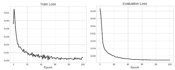
Figure 4: Training (left) and evaluation (right) loss curves. Loss drops to about 70% of the original value.
As shown in Figure 4, training usually asymptotes at around 70% of the original loss value but we do not observe instances of overfitting. Noise in training is present due to the random masking augmentation described in the previous section.
While this demonstrates learning capabilities of the model, MSE loss can be easily reduced by many methods. Due to the similarities between train and evaluation sets (both drawn from data before 2023), overall market trends and high correlation between prices can incentivize a model to learn by memorization of seen patterns.
In the following sections, we evaluate the performance of this model on the test set: data from 2023 onwards.
Accuracy
Recall that at training time, the model is given input_length<=max_context_length=512 data points (with random masking) and tasked to always predict the next output_len=128 many points. Loss is evaluated on these output_len many points.
At inference time, the model is consistently given max_context_length many points (without masking) and tasked to predict the following points. However, we might wish to generate an arbitrary number of future points, not necessarily 128. In our case, we set the prediction horizon_length to be at most 128.
At each step, the model predicts the next horizon_length many points. Accuracy is evaluated on the last output point, where the model is tasked to classify whether the price moves up or down. Accuracy calculation is based on this classification over every inference step.
We observe, in Figure 5, that through fine-tuning, we are able to see consistently better performance over the vanilla pre-trained TimesFM.
As a benchmark, we provide the chance rate, calculated as the accuracy obtained by a random model. For example, if 53% of the price changes in the test set is up, the random model guesses up 53% of the time, and down 47% of the time. Our fine-tuned TimesFM is also able to outperform this benchmark, providing statistical confidence that the improvements we see are not due to random chance.
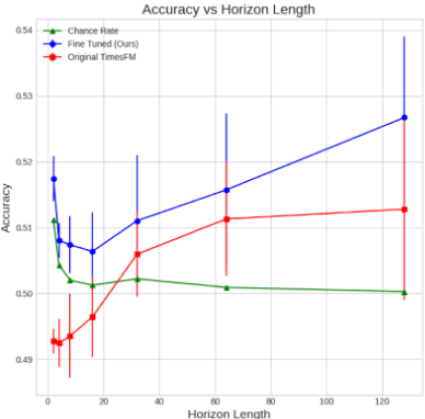
Figure 5: Accuracy against prediction horizon on the test set, containing data from 2023 onwards. Chance rate is defined as the accuracy obtained by a random model that makes predictions based on the overall up:down ratio in the test set.
Mock Trading
In the previous section, we have demonstrated that our fine-tuned model is able to outperform standard benchmarks in price prediction tasks by a reliable and significant margin. In this following section, we develop several trading strategies based on fine-tuned TimesFM and analyze our profits from our trades.
Basic strategy
We begin by describing a trading strategy. In this strategy, we base our trades on close prices only. First, the trader decides on a holding period, we denote this as h=horizon_len. In our model, we set context_length:=c=512. After trading day i the trader input time series \(P_{i-c-1:i}=\{P_{i-c-1}, P_{i-c}, \cdots , P_i\}\) to the model and obtains a prediction for \(P_{i+1:i+h}\). The trader places a buy/sell order on day i+1 and i+h as follows: if \(P_{i+h}>P_{i+1}\), place a buy order on day i+1 and a sell order on day i+h. If \(P_{i+h}< P_{i+1}\), place a sell order on day i+1 and a buy order on day i+h. Repeat this same strategy for all trading days i.
If the trading basket contains a total of \(T\) assets, all orders placed will be worth \(\frac{1}{hT}\). This is such that the L1-norm of orders placed in a day does not exceed 1/h, and that over the holding period does not exceed 1(our total capital). We have to limit the norm of our orders, considering the extreme case where every order during the holding period is a ‘buy’, then we need enough capital to place all the orders.
For testing, we use daily data for S&P500 from 1 Jan 2023 onwards. The returns from executing this strategy can be found in Figure 6.
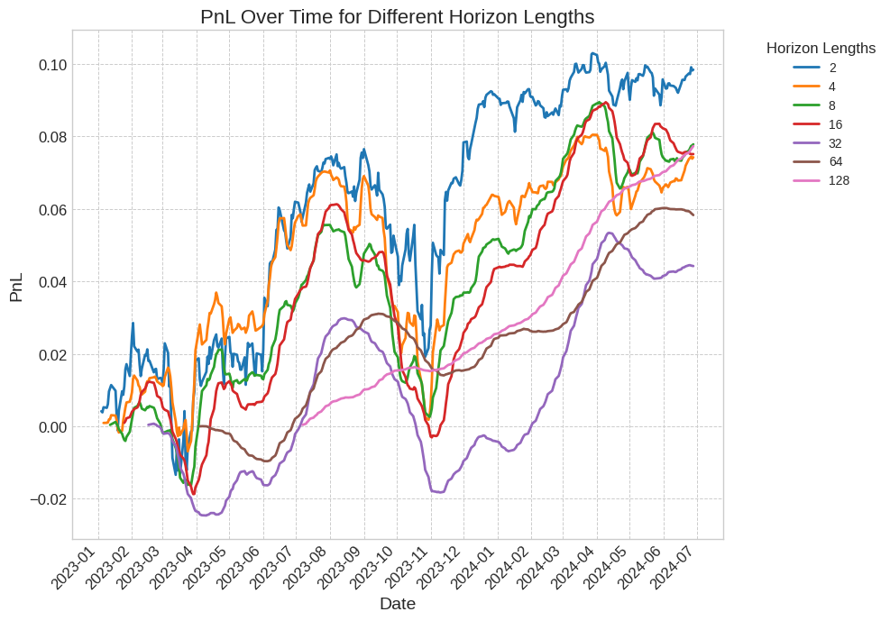
Figure 6: PnL comparisons between different horizon lengths. We achieve positive returns on all horizon lengths. Longer horizon lengths lead to smoother results since the positions change much less frequently, but take longer for the first return to be realized since trades are made in pairs separated by horizon length many days.
Notice that for larger horizon length, one has to wait for a longer duration before the returns are realized. Namely, for a horizon length of 128, one has to wait for 128 trading days before closing the original position, filling both sides of the buy/sell order. This accounts for differences in start points between our graphs. However, these longer horizon lengths give rise to much smoother PnL graphs, due to the much less frequent changes in position. This leads to much lower transaction costs.
A prominent eye-catcher is the sharp drops in the PnL, such as that for horizon 16, that moves together with the overall direction of the market. We propose to remedy this issue by constructing the following market neutral strategy.
Market Neutral Strategy
When constructing our portfolio, we subtract the market mean buy/sell bias (across all tickers) on each trading day. This way, we buy and sell the same amount on both sides. We still ensure that the total L1 norm of trades in one day is 1/h by appropriate normalization. The resulting PnL graph is shown in Figure 7. We also provide useful metrics: sharpe ratio, max drawdown and neutral cost (the trading cost required to zero the returns at the end of the trading simulation).
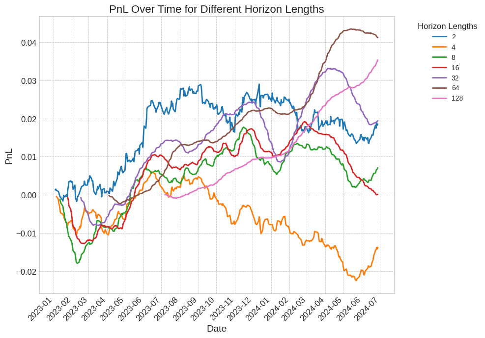
Figure 7: PnL over different horizon lengths using a market neutral strategy. We observe less fluctuations in comparison to Figure 6. Increasing the horizon length leads to smoother PnL curves and lower transaction costs shown in Table 9 and 10.
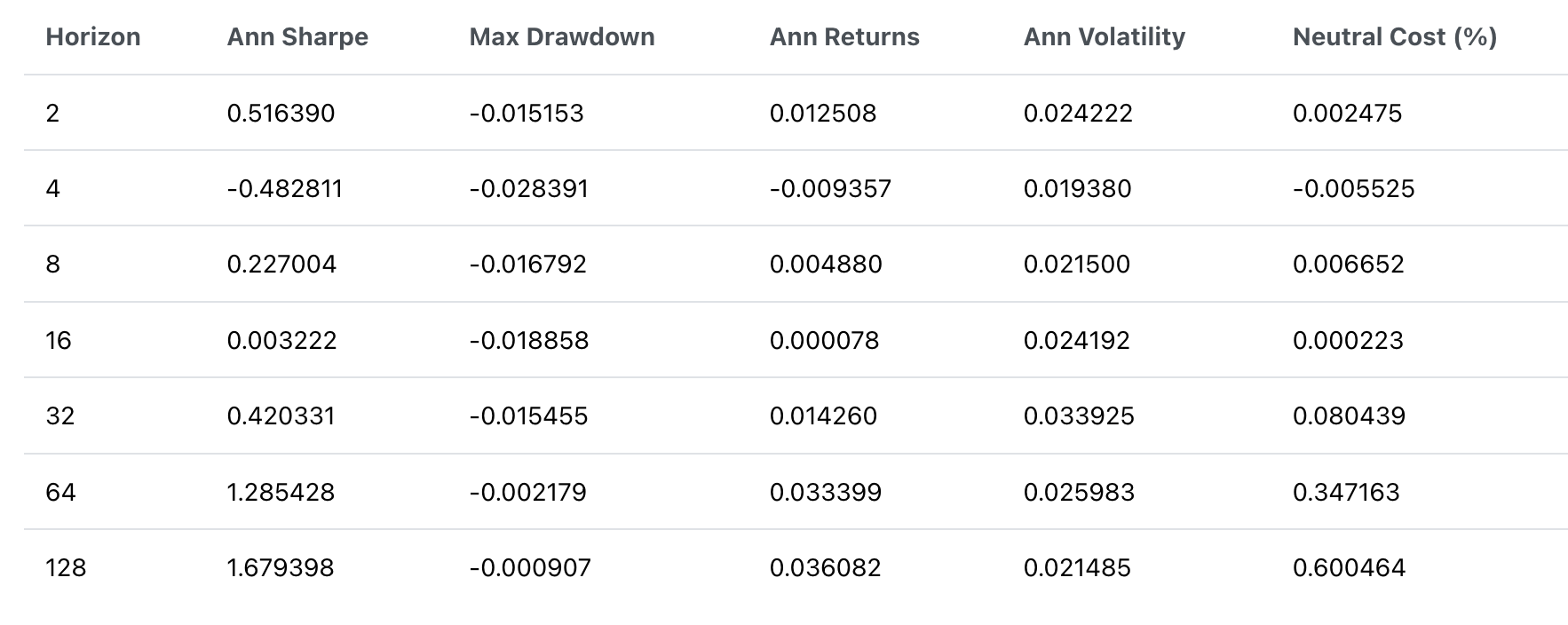
Table 8: Table of evaluation metrics for returns generated by market neutral trading, as shown in Figure 7. Annualized sharpe ratio steadily increases with horizon length as annual returns improve while seeing a reduction in volatility and max drawdown.
Taking a market neutral position allows us to erase the rapid drops due to overall market movement. This is further reflected in the reduced max drawdown and the improved sharpe ratios. We also observe that as we increase the prediction horizon, the slower moving strategies incur lower cost, with the most cost-efficient strategy being executable at a maximum cost of 60 basis points per trade.
Comparison with other models
In this section, we focus on a horizon length of 128 and compare our proposed model against several others. We focus on the market neutral strategy, comparing our proposed fine-tuned TimesFM against the original TimesFM, as well as a random model and an AR(1) model (Box 1970).
For the construction of a random model, we proceed according to the chance rate calculation presented above. Namely, this model is created by first calculating the ratio up:down within the whole dataset, then at each day i, guess the sign of \(P_{i+128}-P_{i+1}\) according to this ratio.
The AR(1) model is an autoregressive model fitted with only the single-difference lagged term. To implement this, on each time series (in the training period) we fit an AR(1) model to obtain the coefficients, then predict on the test dates. Then, mean subtraction is done to turn this into a market neutral strategy.
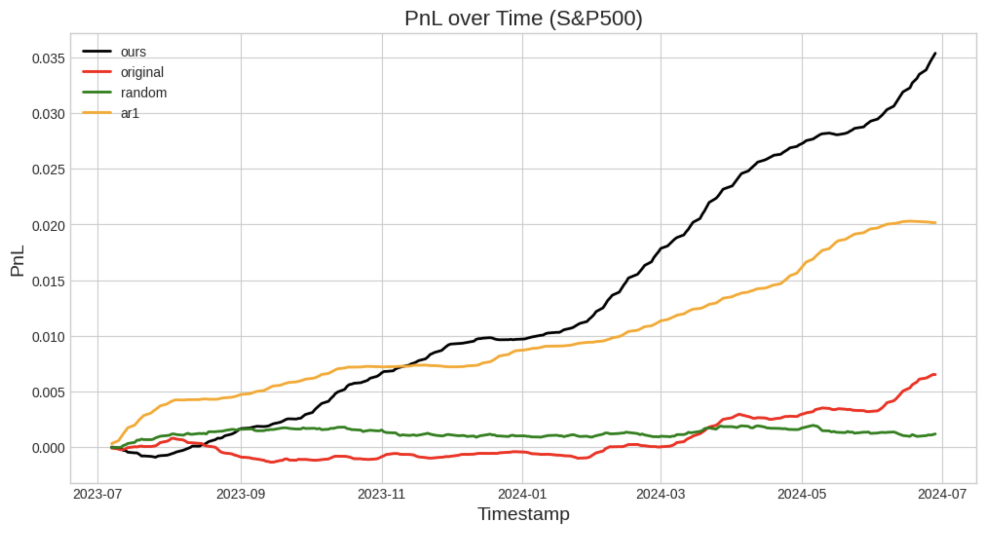
Figure 9: PnL over time of several market neutral strategies when traded on S&P500 stocks. Our fine-tuned TimesFM achieves the highest annual returns of 3.6%.
| Ours | Original TimesFM | Random | AR1 | |
| S&P500 | 1.68 | 0.42 | 0.03 | 1.58 |
| TOPIX500 | 1.06 | -1.75 | 0.11 | -0.82 |
| Currencies | 0.25 | -0.04 | -0.03 | 0.88 |
| Crypto Daily | 0.26 | -0.03 | 0.01 | 0.17 |
Table 10: Sharpe ratio comparisons across different markets. A random model cannot obtain any significant results in a market neutral setting, while our fine-tuned TimesFM shows positive returns on each market, a significant improvement over the baseline TimesFM.
Our model outperforms the original TimesFM on all benchmarks, and the random model cannot make any reliable predictions under a market neutral situation.
However, performance of our model on currencies and crypto is left to be desired. Significantly underperforming the AR1 model. Nonetheless, our fine-tuned TimesFM is still the only model to achieve positive returns on every market.
We can also ascertain the neutral costs of our model in comparison against certain comparison models. We do this in Table 11, aggregating the slippage, transaction cost, and any other expenses into a single cost below.
| Ours | Original TimesFM | Random | AR1 | |
| S&P500 | 0.60% | 0.11% | -0.008% | 0.34% |
| TOPIX500 | 0.14% | -0.24% | 0.02% | -0.18% |
| Currencies | 0.08% | -0.017% | -0.008% | 0.27% |
| Crypto Daily | 0.44% | -0.07% | 0.010% | 0.88% |
Table 11: Neutral cost comparisons, defined as the trading cost (in percentages) required to zero the profits at the end of the trading period. Negative values indicate that the strategy was not making positive profit during the trading period.
So depending on the execution, transaction fees and slippage can add up, and we are only profitable if we keep them under the values as listed in Table 11. Negative values indicate that the strategy was bad to begin with and we would lose money no matter what. We are able to trade up to a cost of 0.60% on S&P500 using our model.
Conclusion
In this blog, we have fine-tuned the SOTA time series foundation model for usage on financial data. By evaluating the loss and accuracy of the model, we see that fine-tuning allows to achieve significantly superior results using the large capacity of TimesFM, outperforming traditional models.
We tested this model using data from 2023 onwards, where we constructed a trading strategy that places buy/sell trades according to the predictions of the model. Through thorough evaluation, we found that a market neutral strategy with a long horizon gives consistently better performance over traditional models, with a sharpe ratio up to 1.68 when traded on S&P500.
We publish our code for reproducibility of results, and hope it inspires future research in this direction.
https://github.com/pfnet-research/timesfm_fin
https://huggingface.co/pfnet/timesfm-1.0-200m-fin
Predicting the market is hard, but we make it easy.