Hello, my name is Huang Baoxi, and I am a first-year master’s student at the Graduate School of Frontier Sciences, the University of Tokyo. My research focuses on ocean informatics and the application of AI to environmental science, particularly using remote sensing and multispectral imagery to analyze coastal organisms.

During this internship, my topic is “Maintenance of LLM training dataset”, with a specific focus on deduplication to improve dataset quality.

2. Background

2.1 What is Duplicated Data for LLMs?

As the volume of data has grown year by year, large language models (LLMs) have benefited from increasingly rich training corpora. However, this growth also brings a significant challenge: duplicated data. Figure 1 illustrates this issue. Although the proportion of duplicated data (in red) may appear relatively small, the scale of modern datasets is on the order of 10^10, meaning even a small percentage translates into an enormous number of repeated samples.

Duplicated data can arise in many ways. Research papers and industry reports are often republished in slightly modified forms, while webpages may contain nearly identical content across different social media platforms or exhibit HTML layout variations introduced during web crawling. In addition, the same scientific publication can yield different outputs when processed by different PDF parsing tools. In all of these cases, the underlying information is effectively the same, yet it appears multiple times in the dataset.

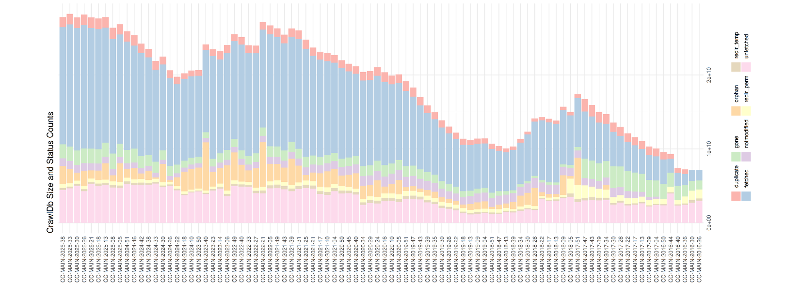
Figure 1. The amount of annual data size from 2016 (right) – 2025 (left). The red part shows the duplication portion [1].

2.2 Why It Matters to LLMs

Duplicated data increases the overall size of the dataset, which directly translates into longer processing time, higher memory consumption, and greater disk usage for storage. Beyond these engineering costs, duplicated data also undermines the effectiveness of training. A growing body of research has shown that the quality of training data is as important as its quantity [5][8]. Table 1 illustrates this point by comparing model performance under different deduplication strategies. With careful deduplication, models achieve similar or better accuracy while training on 13–41% fewer tokens. This reduction not only saves computational resources but also shortens the time required to reach convergence. Another important aspect is the impact on data distribution. Deduplication alters the balance of the dataset, sometimes causing the model to overfit on certain topics rather than learning to generalize across diverse domains. Since one of the goals of LLMs is to perform robustly across a wide variety of tasks, maintaining the right balance between removing redundancy and preserving diversity is essential.

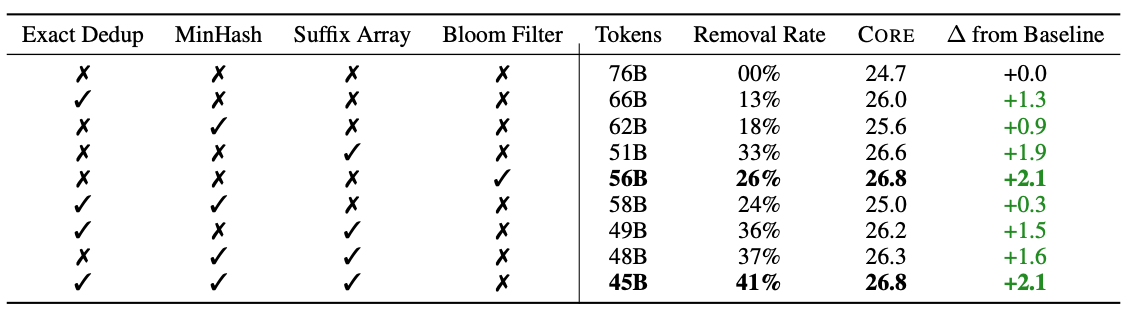
Table 1. Evaluation of Core score (accuracy on various downstream tasks) on different combinations of deduplication methods [5]

2.3 Current Deduplication Method – MinhashLSH

The presence of such redundancy not only wastes storage and computational resources but can also bias models and reduce their generalization ability. To address this problem, it is necessary to establish a clear definition of what it means for two texts to be considered duplicates. A common solution is to use Jaccard similarity, which quantifies the overlap between two sets of tokens [10]. By setting a threshold T, two texts are classified as duplicates if their Jaccard similarity exceeds this value. The mathematical formula is expressed as follows:

\(J\left(A,B\right)=\frac{\left|A\cap B \right|}{\left|A\cup B \right|}\)

In this way, the notion of duplication is transformed from an ambiguous, subjective judgment into a measurable criterion.

However, in large datasets, computing the exact Jaccard similarity between two sets can be prohibitively time-consuming. To solve this problem, Minhash provides an efficient approximation approach to deduplicate through permuting the order of two sets to produce MinHash signature[9]. By applying multiple random permutations, the probability of two signatures is equal approximates the Jaccard Similarity.

MinHashLSH builds upon the MinHash algorithm by introducing a locality-sensitive hashing (LSH) scheme [7]. The motivation is straightforward: without LSH, MinHash would still require comparing every pair of documents to evaluate similarity, which results in quadratic cost and quickly becomes infeasible on large datasets. The schematic is shown in Figure 2. Given a set of MinHash signatures, we can construct a signature matrix in which each column corresponds to a document and contains all of its MinHash values. To efficiently identify potential duplicates, the rows of this matrix are divided into bands of size 𝑏, determined by the desired Jaccard similarity threshold 𝑇. Each band is then hashed into buckets. Documents that fall into the same bucket are treated as candidate pairs, significantly reducing the number of comparisons needed. In this way, LSH concatenates a series of potential duplicate pairs while avoiding exhaustive pairwise comparisons.

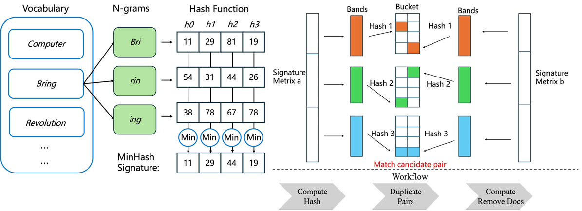
Figure 2. Schematic of LSH

From the perspective of time complexity, LSH reduces the quadratic cost of naive MinHash comparisons to something far more manageable by focusing only on candidate pairs within buckets. However, the process of matching candidate pairs cannot be easily parallelized which limits the scalability in practice. Besides, the prefix-tree–like structure will introduce a significant challenge in space complexity since MinHashLSH requires storing signatures for all documents. While these signatures are far smaller than the original documents, at the scale of billions of documents the storage requirements grow dramatically. For example, in their experiments a dataset of 5 billion documents required approximately 23 TB of space[3]. Thus, while the method is efficient in reducing time complexity, it still incurs an 𝑂(𝑛) cost in terms of storage.

2.4 Current Issue in LSH-based deduplication

While MinHashLSH provides a principled way to reduce the quadratic cost of pairwise comparisons and makes large-scale deduplication feasible in theory, its practical application reveals important limitations. The efficiency gains in time complexity come at the cost of significant memory overhead, since all document signatures must still be stored and processed when computing duplicate pairs in the workflow. When moving from theoretical design to real-world deployment, these memory requirements quickly become the bottleneck.

Figure 3 illustrates the memory footprint and the challenges we encountered when applying LSH-based deduplication to a 600 GB dataset on AWS. In this experiment, we have used several computational instances to accomplish it. Our initial attempt used a spot instance with 30 GB of memory, but the process failed with out-of-memory (OOM) errors. We then upgraded to a larger on-demand instance with 64 GB of memory, yet the problem persisted. Ultimately, we were forced to reduce parallelism from 4–8 processes down to a single process. While this solution worked, it significantly increased the runtime to about one hour. For a 600 GB dataset, this trade-off was tolerable, since the cost of a single hour on AWS is relatively modest. However, the situation becomes much more critical when considering realistic scales for LLM training datasets. Modern corpora can easily reach 600 TB or more. At that scale, a one-hour runtime scales into weeks, and the associated compute cost grows dramatically. Moreover, deduplication is not a one-time operation. Since web data is continuously updated, new data must be deduplicated regularly, compounding the cost over time.

These challenges highlight a pressing need for memory-efficient deduplication algorithms. Without addressing the memory bottleneck, LSH-based deduplication cannot be feasibly scaled to the size and frequency required for large-scale LLM training.

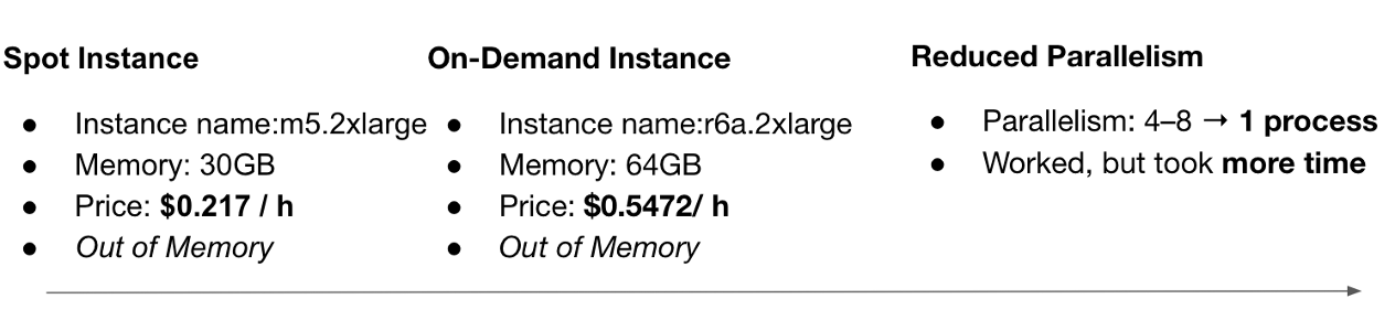
Figure 3. The footprint of LSH-deduplication on cloud usage

3 Methodology

3.1 Bloom Filter for Data Deduplication

The Bloom filter is a space-efficient probabilistic data structure originally proposed by Burton Howard Bloom in 1970, which determines whether an element belongs to a set [6]. More recently, researchers have incorporated this method into deduplication pipelines to improve the efficiency of MinHashLSH [3]. Building on this line of work, we explored Bloom filters in our deduplication experiments to reduce both memory usage and processing time on AWS.

The key idea of Bloom Filter is instead of storing full document representations, the Bloom filter encodes documents as bits in an array. When a new document is processed, multiple hash functions compute index positions, and the corresponding bits in the array are set to 1, as illustrated in Figure 4. If the same document (or one hashed to the same positions) is encountered again, the filter detects it immediately and discards it without requiring additional storage so the workflow can be simplified into two steps: computing hash and Bloom filter processing. Because of this design, Bloom filters may produce false positives (flagging a document as duplicate when it is not) but never false negatives (failing to detect an actual duplicate). In other words, recall is preserved while precision may slightly decrease.

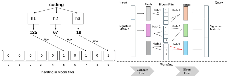
Figure 4. Illustration of Bloom Filter (left) and schematic of LSHBF-deduplication (right).

From the parallel perspective, it is natural to assign each band to its own Bloom Filter rather than querying all bands through an index as in LSH, making it much easier to achieve parallelization. From a complexity perspective, Bloom filters are highly memory-efficient. The total space usage depends only on the size of the bit array 𝑛, giving a space complexity of O(𝑛). Each membership check and insertion requires only 𝑘 hash operations, where 𝑘 is a constant number of hash functions, making the per-operation cost effectively 𝑂(1). The choice of 𝑛 and 𝑘, which balances memory usage against the false positive rate, is described in the Appendix. In addition, the false positive rate (FP) serves as a tunable parameter that controls the trade-off between memory usage and accuracy. Since this parameter is explicitly configurable, we can adjust it to preserve results comparable to LSH while avoiding significant additional cost [3].

The basic pseudo-code is as follows:


for doc in docs:
    # Query
    if doc in bloom_filter:
        discard
    else:
        # Insert
        bloom_filter.add(doc)

To further reduce memory usage and accelerate runtime, we implemented this approach using rBloom[12], a high-performance Bloom filter library written in Rust. rBloom is significantly faster than other available libraries, making it well suited for replacing traditional LSH in large-scale deduplication pipelines.

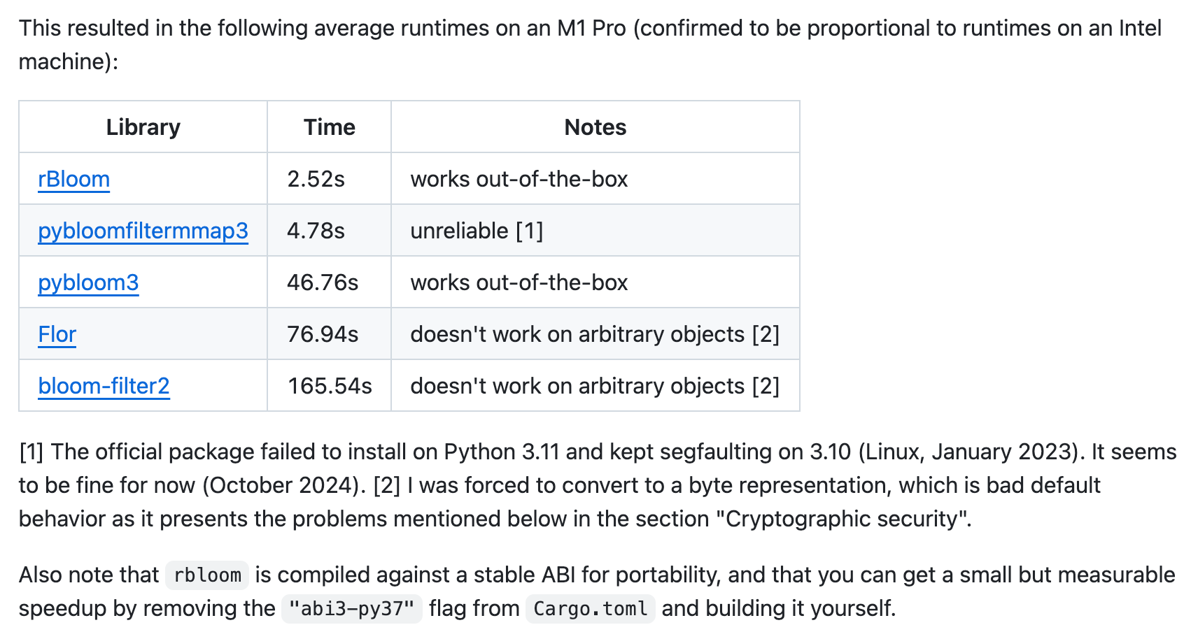
Figure 5. Leaderboard of Bloom Filter implementation [12]

3.2 Data Loader for Hash Value

The pseudo-code illustrates the basic process of how a Bloom filter detects duplicate documents. However, a bottleneck arises because all hash values for each band are loaded into memory simultaneously, leading to excessive memory consumption. To address this issue, I developed a data loader that processes hash values in batches. Instead of loading the entire band at once, the Bloom filter iterates through smaller batches of hash values. Each batch is loaded only when needed and is removed from memory once processing is complete, thereby reducing overall memory usage.

4 Experiment

4.1 Dummy Set Construction

To validate the correctness of our LSHBF workflow, we first needed a dataset with reliable ground truth labels. Since such deduplication benchmarks are difficult to obtain, we constructed a manually well-structured dummy dataset. This controlled dataset allowed us to systematically test and evaluate the method under known conditions. We began by using an LLM to generate 𝑛 unique documents, ensuring that each document was completely distinct from the others. We then introduced duplicates by applying three fine-grained patterns: copy, delete, and modify, with ground truth labels explicitly recorded. In total, the dummy dataset contained 1,500 documents. While this dummy set provided a controlled environment to validate correctness, its small scale was insufficient for evaluating resource usage and scalability. To address this, we turned to a larger public dataset as shown in Figure 6 and constructed subsets ranging from 10 GB to 40 GB by duplicating documents.

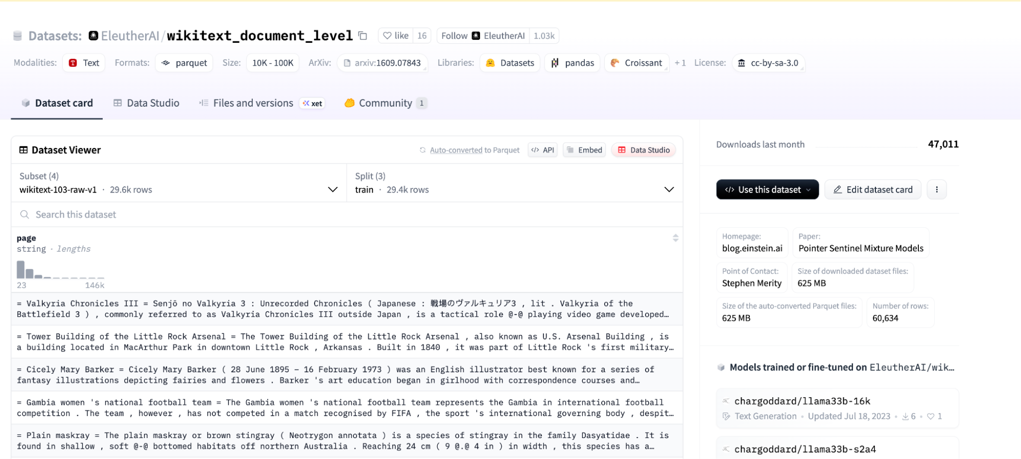
Figure 6. Public dataset in Hugging Face [11]

5 Results

5.1 Precision, Recall and F1 score

When evaluating a deduplication method, three key metrics are considered: precision, recall, and computational performance. Precision measures how many of the predicted duplicates are actually correct. Low precision indicates excessive false positives, which is harmful because it unnecessarily reduces the size of the training dataset. Recall measures how many of the true duplicates are successfully identified. Low recall indicates excessive false negatives, which leaves duplicate content in the dataset and can negatively affect learning, even leading to degenerate behavior such as memorization. The mathematical definitions of precision, recall, and F1 score are as follows:

\(\text{Precision} = \frac{TP}{TP + FP}\)

\(\text{Recall} = \frac{TP}{TP + FN}\)

\(F1 = \frac{2 \cdot \text{Precision} \cdot \text{Recall}}{\text{Precision} + \text{Recall}}\)

In this project, we place greater emphasis on recall, since it directly influences the distribution of the dataset. Precision, on the other hand, is less critical: if we lose some non-duplicate data due to false positives, this can be compensated by simply adding more raw data to the corpus.

The results on the dummy dataset are summarized in Table 2. Both LSH and LSHBF achieved high performance, maintaining strong precision and recall with comparable F1 scores. Notably, LSHBF reached higher precision, ensuring that no false positives were introduced, while recall remained at a similar level to LSH. As shown in wall clock and memory usage in Table 2, our approach maintains high accuracy while reducing wall clock time. Although the dummy dataset is too small to provide a precise evaluation of memory usage due to overhead effects, the results still fall within an acceptable range. A more pronounced comparison of memory efficiency can be observed in Section 5.3 .

Table 2. Deduplication accuracy comparison between LSH and LSHBF

	Precision	Recall	F1	Wall clock (s)	Memory usage (MiB)
LSH	0.9967	0.5412	0.7015	17.31	1.953125
LSHBF	1.0	0.5341	0.6963	13.98	2.07421875

5.2 The Probability of Detecting Candidate Pairs

As mentioned in Section 4.1, we constructed a dummy dataset with different duplication patterns, and the distribution of Jaccard similarity is shown in Figure 7. We set the threshold at 𝑇=0.8. This means that whenever the Jaccard similarity between two documents exceeds 0.8, they are regarded as duplicates. Most of the documents cluster near 1. Given the number of band 𝑏, band size 𝑟, and the false positive rate, we can plot a comparison curve to show the theoretical and actual probability of detecting at least one candidate pair across the two deduplication methods. The two actual curves align closely with each other and show only a slight deviation from the theoretical value, which is well within an acceptable range and consistent with our expectations. Figure 8 further illustrates the prediction distributions of LSH and LSHBF on this dummy dataset, confirming that the difference in deduplication accuracy between the two algorithms is minimal.

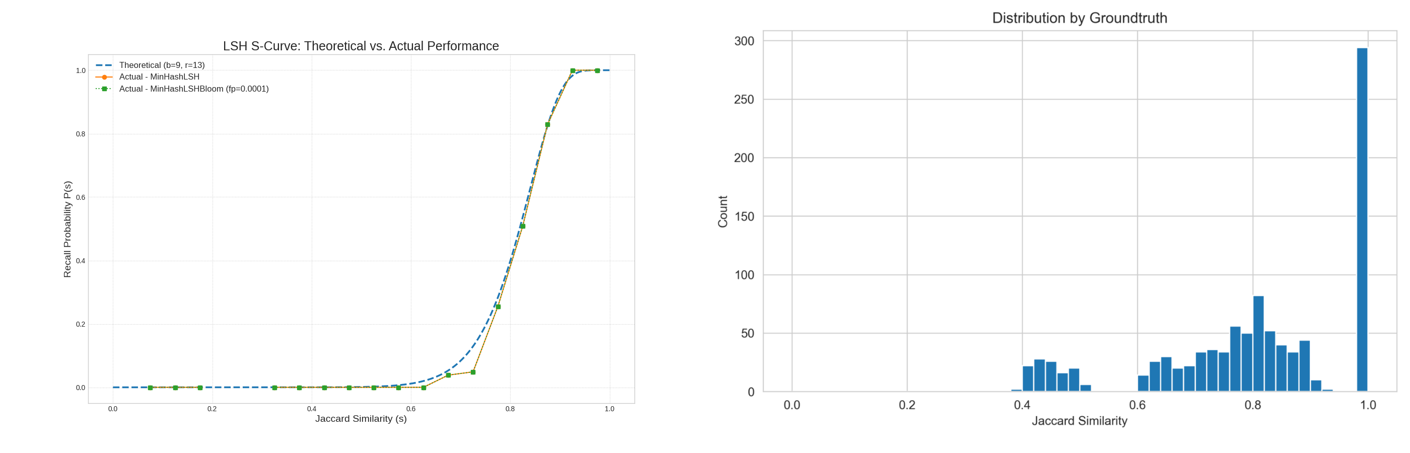
Figure 7. The S-Curve (left) and the distribution of dummy dataset (right)

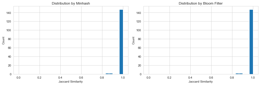
Figure 8. Distributions from dummy dataset

In Figure 9, we simulate more realistic scenarios by constructing distributions that reflect real-world conditions. The two distributions range from 0.3 to 0.9, and the results show that no candidate pairs are detected by either algorithm. This indicates that no false positive errors occur within these distributions, further confirming the robustness of both methods.

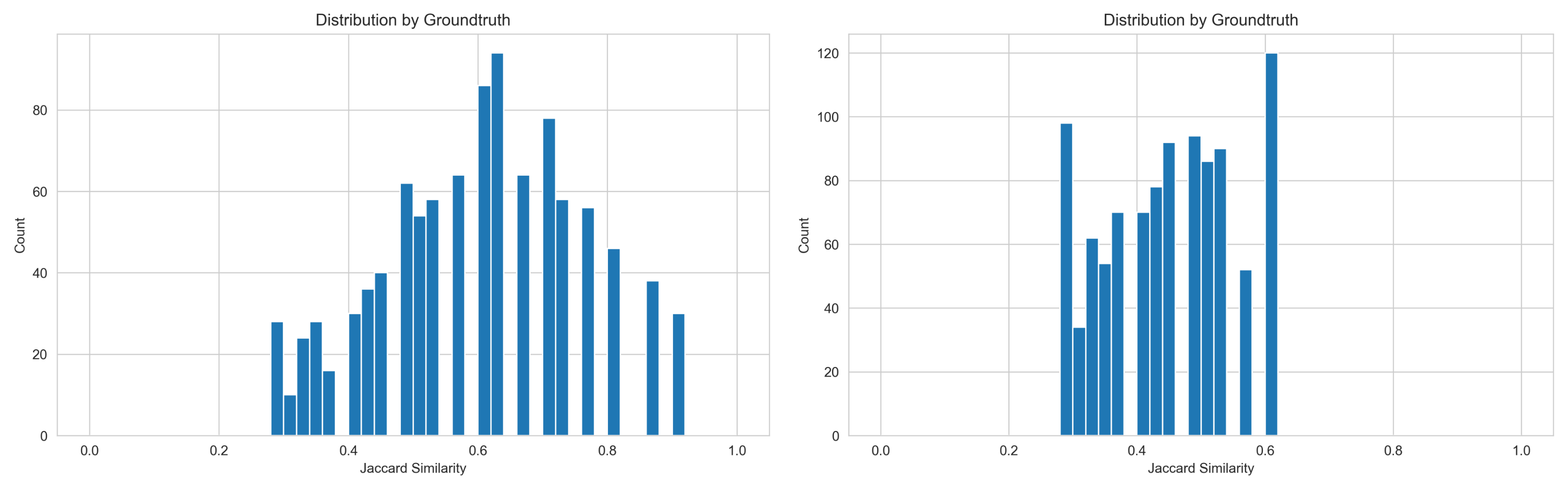
Figure 9. Different Distributions from dummy dataset

5.3 Wall-clock Time, Memory Usage and Agreement

When evaluating the accuracy of LSHBF on large datasets where ground truth labels are unavailable, we adopt an agreement metric, which measures the prediction gap between different deduplication algorithms. This allows us to indirectly assess accuracy by checking how closely LSHBF aligns with established baselines. The formula can be described as follow:

\(\text{Agreement} = \frac{1}{n} \sum_{i=1}^{n} \mathbf\! [ y_{A,i} = y_{B,i}]\)

Our expectation is that LSHBF can significantly reduce wall-clock time and memory consumption while maintaining agreement at a comparable level. As shown in Figure 11 and 12, the results validate this expectation: LSHBF achieves a 38.4% reduction in processing time and an 87.2% reduction in memory usage compared to the baseline method, while preserving strong agreement in predictions.

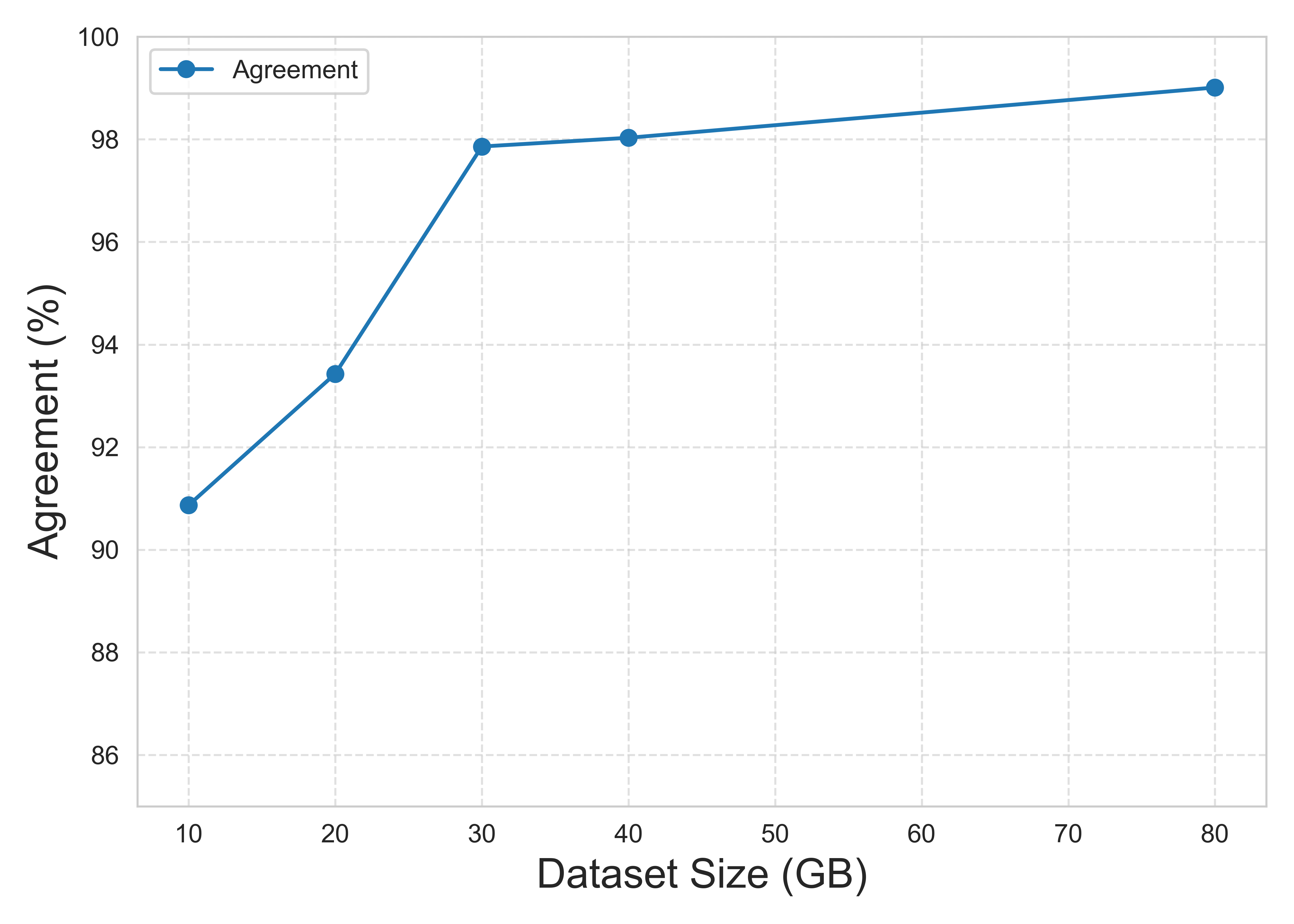
Figure 10. Agreement of LSHBF with LSH

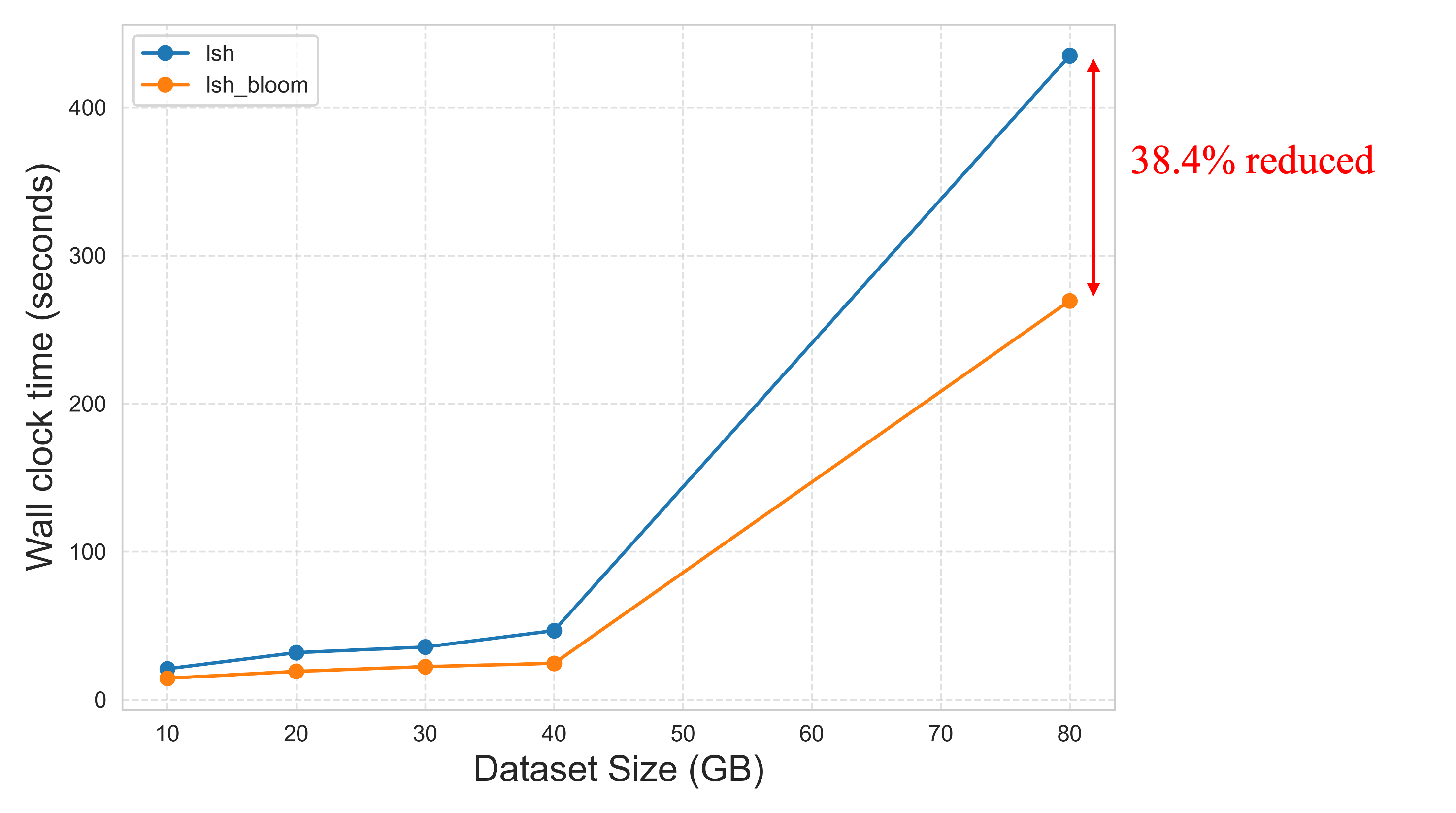
Figure 11. Wall clock time consumption of LSH and LSHBF

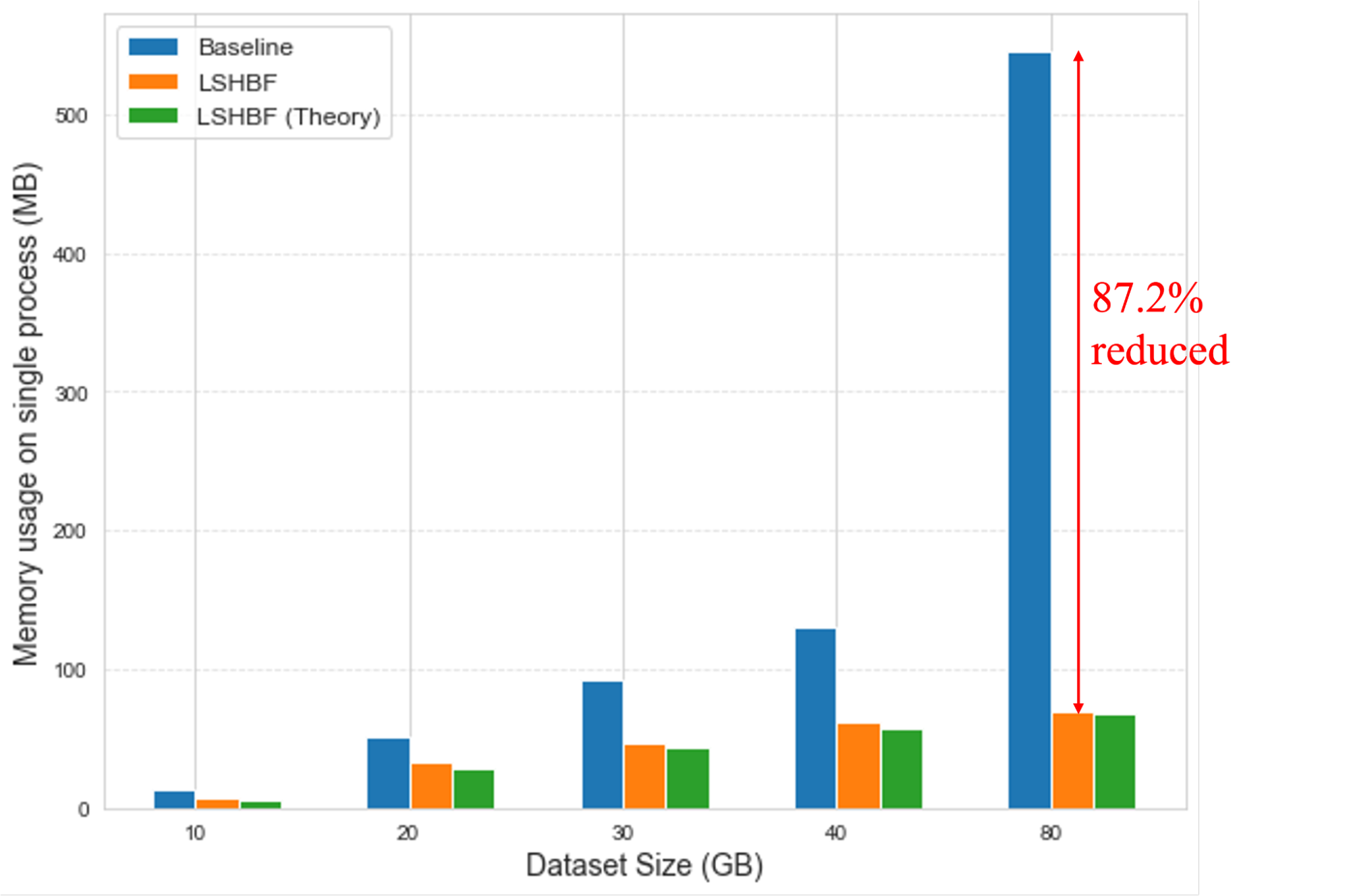
Figure 12. Comparison of memory usage by LSH(baseline) and LSHBF. The green bar shows the theoretical value by using Bloom Filter.

6 Conclusion

In this project, we explored the effectiveness of LSHBF-based deduplication, which preserves comparable accuracy while requiring significantly fewer computational resources in terms of wall-clock time and memory consumption. To validate its accuracy, we constructed several dummy datasets with different distributions. Across these datasets, LSHBF achieved results almost identical to LSH in terms of precision, recall, and F1 score. On larger datasets, such as an 80 GB corpus, LSHBF maintained high agreement with baseline methods while reducing memory usage by 87.2% and processing time by 38.4%.

Although Bloom filters demonstrated clear performance advantages in the deduplication pipeline, a major bottleneck remains: reading and managing the hash signatures still consumes substantial memory, which may prevent us from fully overcoming OOM issues observed in Figure 3. To address this challenge, our future work will focus on further optimizing the hash-loading stage with less memory needed. In addition, when resources permit, we plan to train large-scale models on the deduplicated datasets to more rigorously evaluate the accuracy of the deduplication process and the robustness of the proposed algorithm.

Appendix

In this project, we explored a memory-efficient alternative to MinHashLSH by integrating Bloom filters into the deduplication pipeline. For each band of the MinHash signature matrix, we instantiate a dedicated Bloom filter. Rows of MinHash signatures within a band are processed through 𝑘 independent hash functions, which map them into integer indices. These indices are then inserted into the Bloom filter of fixed size 𝑚. In this way, duplicate signatures can be identified without the need to store explicit prefix-tree structures, dramatically reducing memory usage. The optimal values of 𝑚 and 𝑘 are determined analytically based on the number of documents 𝑛 and the target false positive probability 𝜀:

\(\mathrm{m}=-\frac{\mathrm{n} \ln \varepsilon}{(\ln 2)^{2}}\)

\(\mathrm{k}=\frac{\mathrm{m}}{\mathrm{n}} \ln 2\)

In all of our experiments, we set the false positive probability to 𝜀 = 1e-5, striking a balance between memory efficiency and accuracy.

As mentioned in Section 3.1, the Bloom Filter may produce FP but never FN. The impact of FP can be reduced to a negligible level through careful parameter tuning. Given b bands with r size of each band, the false positive overhead introduced by Bloom filters can be expressed as:

\(\mathrm{P}_{effective}=1-(1-\varepsilon)^b\)

Reference

[1] Statistics of Common Crawl Monthly Archives: https://commoncrawl.github.io/cc-crawl-statistics/plots/crawlermetrics

[2] Locality Sensitive Hashing (LSH): https://www.pinecone.io/learn/series/faiss/locality-sensitive-hashing

[3] Khan et al., (2024): Lshbloom: Memory-efficient, extreme-scale document deduplication. arXiv preprint arXiv:2411.04257.

[4] Bloom Filters 101: The Power of Probabilistic Data Structures: https://medium.com/@sylvain.tiset/bloom-filters-101-the-power-of-probabilistic-data-structures-ef1b4a422b0b

[5] Li, J., Fang, A., Smyrnis, G., Ivgi, M., Jordan, M., Gadre, S. Y., … & Shankar, V. (2024). Datacomp-lm: In search of the next generation of training sets for language models. Advances in Neural Information Processing Systems, 37, 14200-14282.

[6] Bloom, B. H. (1970). Space/time trade-offs in hash coding with allowable errors. Communications of the ACM, 13(7), 422-426.

[7] Leskovec, J., Rajaraman, A., and Ullman, J. D. Mining of Massive Datasets, 3rd Edition, chapter 3: Finding similar items, pp. 73–130. Cambridge University Press, 2014. http://www.mmds.org.

[8] Lee, K., Ippolito, D., Nystrom, A., Zhang, C., Eck, D., Callison-Burch, C., and Carlini, N. Deduplicating training data makes language models better, 2021. Preprint arXiv:2107.06499.

[9] Broder, A. Z., Charikar, M., Frieze, A. M., and Mitzenmacher, M. Min-wise independent permutations. In 30th ACM Symposium on Theory of Computing, pp. 327–336, 1998.

[10] Murphy, A. H. (1996). The Finley affair: A signal event in the history of forecast verification. Weather and forecasting, 11(1), 3-20.

[11] EleutherAI/wikitext_document_level https://huggingface.co/datasets/EleutherAI/wikitext_document_level

[12] rBloom https://github.com/KenanHanke/rbloom

Area

Machine Learning / Deep Learning

Tag