This blog was originally written by Kei Ishikawa (@kstoneriv3), summarizing his work during his internship at Preferred Networks developing Optuna.

In this blog post, we introduce the recent update in Optuna’s default optimization algorithm. This update enables better hyperparameter optimization performance with Optuna.

If you’re new to Optuna, here’s the quickstart on Colab, v1 release announce post!

TL;DR

• Optuna has been using “independent” TPE as the default optimization algorithm but could not capture the dependencies of hyperparameters
• In order to take the dependencies of hyperparameters into considerations, we updated the “independent” TPE to “multivariate” TPE
• In our benchmarks, “multivariate” TPE found better solutions with less computational budgets than “independent” TPE

Usage

To use multivariate TPE, you need Optuna of version 2.2.0 or later. Once you have that installed, just turn on the `multivariate` flag of the `TPESampler` as follows.

 
# In this example, we optimize a quadratic function.
import optuna

def objective(trial):
    x = trial.suggest_float("x", -1, 1)
    y = trial.suggest_float("y", -1, 1)
    return x ** 2 + y ** 2

# We use the multivariate TPE sampler.
sampler = optuna.samplers.TPESampler(multivariate=True)

study = optuna.create_study(sampler=sampler)
study.optimize(objective, n_trials=100)

TPE: A Hyperparameter Optimization Algorithm

Before diving into the details of the update from “independent” to “multivariate”, let us first review the TPE algorithm, which is Optuna’s default optimization algorithm.

TPE stands for the Tree-structured Parzen Estimator [1] and is a hyperparameter optimization algorithm. Hyperparameter optimization can be formulated using a framework of Bayesian optimization [2]. In the Baysian optimization, we minimize (or maximize) an unknown objective function f(x) with respect to a vector x (hyperparameter) by iteratively selecting x and observing noisy objective value y = f(x) + ε, as in the following algorithm.

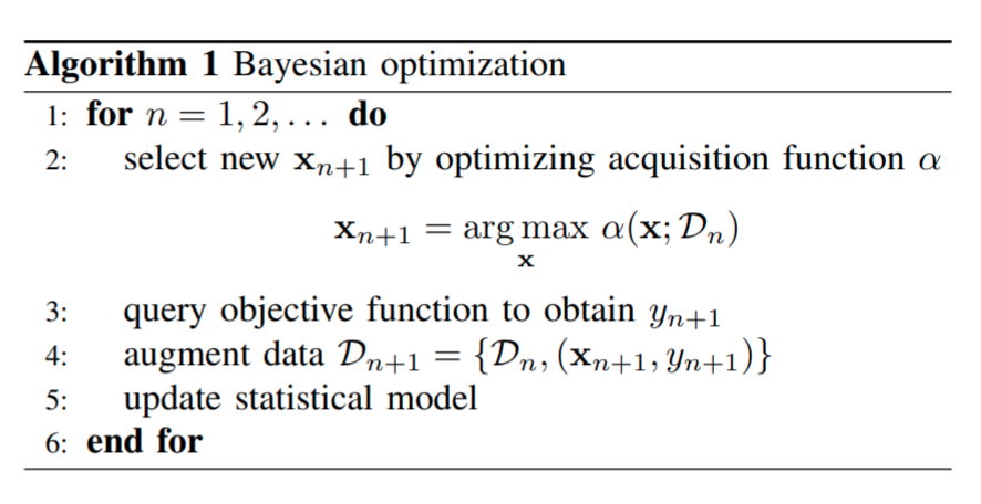
Pseudo code of Bayesian optimization from [2].

As can be expected from its name, the TPE algorithm uses Parzen window estimators as its building component. The Parzen window estimator is a statistical model for density estimation, which is also called the kernel density estimator. Intuitively speaking, the Parzen window estimator (in right figure) is a smoothed version of the histogram of relative frequency (in the left figure).

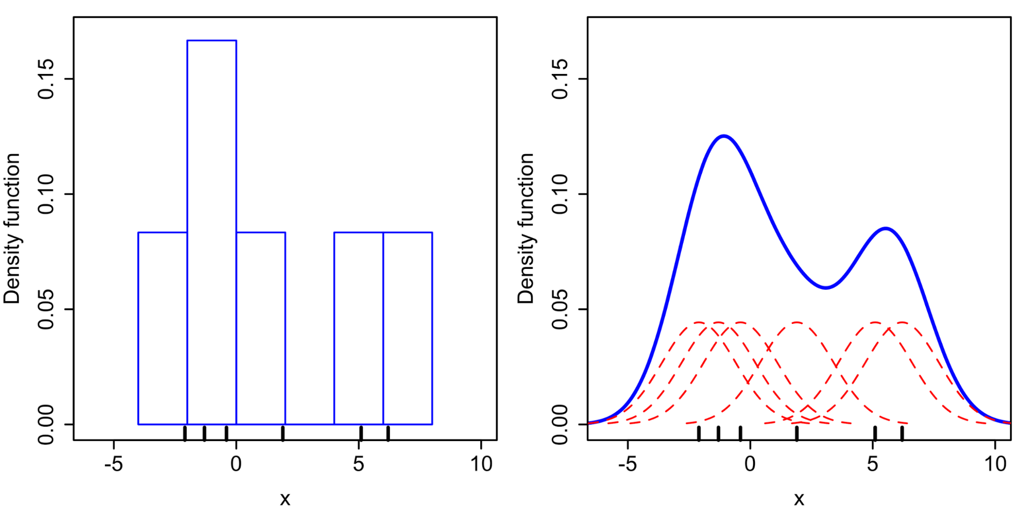
A comparison of histogram and Parzen window estimator taken from [3].

In the TPE algorithm, Parzen window estimators are used to estimate the densities of good hyperparameters and bad hyperparameters. We divide the previously evaluated hyperparameter configurations into two groups by thresholding the objective values at y*. Then fitting the Parzen window estimator to each group, we construct density of good hyperparameters l(x) = p(x|y<y*) and bad hyperparameters g(x) = p(x|y>y*). Using these density estimates, TPE picks the next hyperparameter to try as the maximizer of the density ratio l(x)/g(x). Intuitively, TPE is selecting the hyperparameter configuration which is most likely to be good and least likely to be bad.

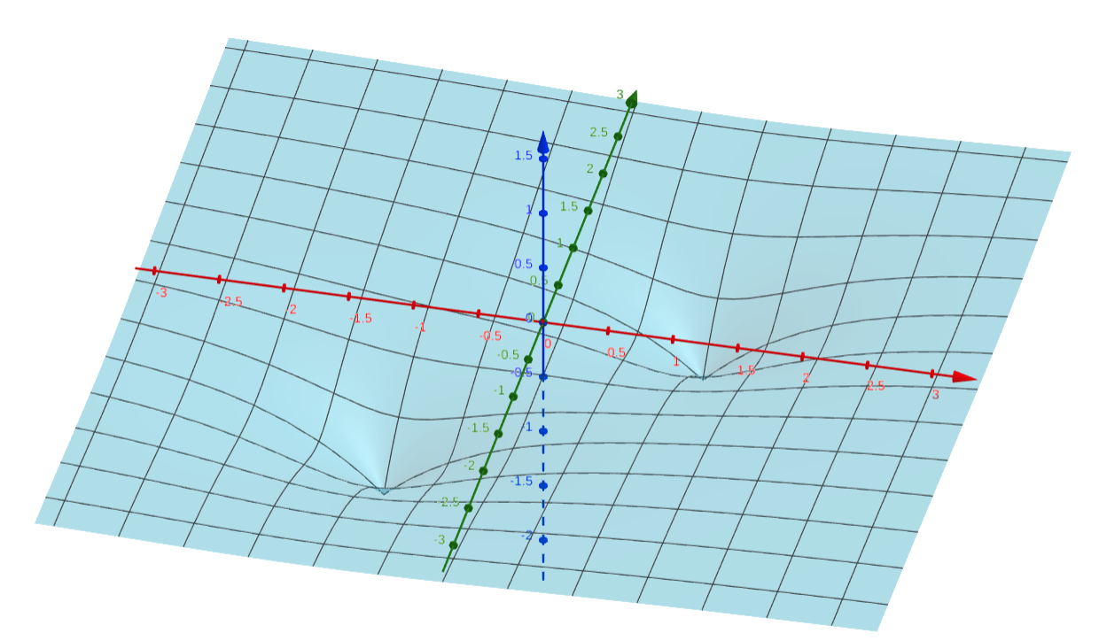
An example of objective function with two minima.

For example, when we have a function with two different minima as in the figure above, hyperparameters are sampled by the (multivariate) TPE as in the following animation. The heat map of the animation shows the density ratio l(x)/g(x). We can see that as the optimization progresses, near the optimal solution, the density ratio becomes high and more hyperparameters are sampled.

An animation of the heat map of density ratio and sampled hyperparameters in the during hyperparameter optimization.

From “independent” TPE to “multivariate” TPE

Finally, let us discuss why we need “multivariate” TPE.

Before this update, Optuna only supported an independent TPE, which ignores the dependencies among parameters. For example, in independent TPE, when we have three dimensional hyperparameter x = (x1, x2, x3), the densities of good / bad hyperparameters are estimated as the product of univariate Parzen window estimator as

l(x) = l1(x1) * l2(x2) * l3(x3) and
g(x) = g1(x1) * g2(x2) * g3(x3),

where l1, l2, … are the parzen window estimators of densities of x1, x2, … .

Multivariate TPE sampler, on the other hand, models l(x) and g(x) directly using single multivariate Parzen window estimators. Thus, the multivariate TPE can capture dependencies among parameters. As the multivariate TPE uses more expressive models for estimating the density ratio, we expected “multivariate” TPE to perform better than “independent” TPE and therefore decided to support multivariate TPE.

A keen reader might notice that the example above with two minima illustrates a scenario where two parameters are clearly correlated. The optimal x0 depends on x1 and vice versa. This is where the multivariate TPE comes into play.

Benchmark Results

To compare the performance of multivariate TPE against the independent TPE, we took benchmarks of both algorithms.

The benchmark problem was the hyperparameter optimization of a neural network on the HPO-bench dataset [4], where the optimizer can evaluate the objective value at 100 different hyperparameters. For taking the benchmarks, we used a benchmark tool kurobako and repeated 100 experiments per each benchmark.

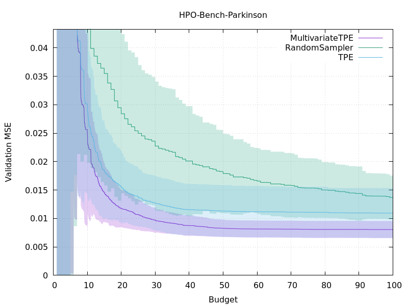
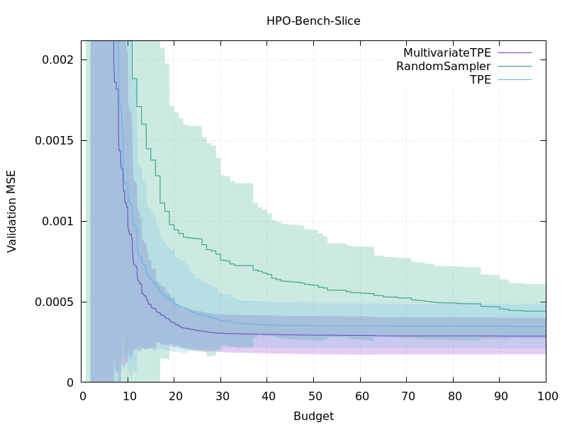
Plots of the performance of different optimization methods.

The above figures show the objective values during hyperparameter optimization. The horizontal axes show the number of hyperparameters evaluated during the optimization. The multivariate TPE corresponds to the purple line and the blue one indicates the independent TPE. The green line represents random sampling and is added just for reference. As we expected, the multivariate TPE outperformed the independent TPE and the multivariate TPE is finding better solutions more quickly than the independent TPE. Moreover, in other benchmarks not listed, we observed similar results; the multivariate TPE performed better than the independent TPE to some extent.

Conclusion

We implemented multivariate TPE in Optuna to take into consideration the dependencies of hyperparameters during optimization. This update will improve the optimization performance and will enable more efficient hyperparameter optimization with Optuna.

Head over to GitHub to try it out!

Future Works

As Optuna is already equipped with powerful pruners, a combination of those pruners with the multivariate TPE would be a promising next step. Indeed, BOHB [5] combines multivariate TPE with the Hyperband pruning algorithm and competitive performance is reported. However, so far in our experiments, no significant improvement was observed by this combination. We consider this is because of the difference in the implementation details. Thus, the refinement of the current implementations of the Hyperband and the multivariate TPE with a view to combining them will be an important future work.

References

[1] Algorithms for Hyper-Parameter Optimization (NIPS 2011), http://papers.nips.cc/paper/4443-algorithms-for-hyper
[2] Taking the human out of the loop: A review of Bayesian optimization. Proceedings of the IEEE 2015, https://ieeexplore.ieee.org/document/7352306
[3] Figures taken from “Kernel density estimation (Wikipedia, retrieved on 20 Sep. 2020)”, https://en.wikipedia.org/wiki/Kernel_density_estimation
[4] Tabular Benchmarks for Joint Architecture and Hyperparameter Optimization. Preprint 2019), https://arxiv.org/abs/1905.04970
[5] BOHB: Robust and Efficient Hyperparameter Optimization at Scale (ICML 2018), http://proceedings.mlr.press/v80/falkner18a.html