Density Functional Theory (DFT) calculations are among the most accurate and widely used simulation techniques for investigating the electronic structure of matter. In recent years, with the rapid rise of artificial intelligence (AI) in materials science, DFT has become the standard for generating high-quality datasets used to train neural network architectures that can predict material properties.

Neural Network Potentials (NNPs) offer a faster alternative to direct DFT calculations. However, generating the training datasets with DFT remains the most important bottleneck, since DFT is computationally demanding. Therefore, making DFT calculations more efficient without significantly compromising accuracy would greatly benefit the entire workflow of AI-driven materials discovery.

One promising approach is to improve the quality and efficiency of pseudopotentials, which are central to plane-wave DFT calculations.

What Are Pseudopotentials and Why Are They Used?

DFT calculations are based on solving the Kohn–Sham equations self-consistently:
\[H_{\rm KS} \psi_i(r) = \varepsilon_i \psi_i(r),\]

where the Kohn–Sham Hamiltonian is

\[HKS = -\frac{\hbar^2}{2m} \nabla^2 + V_{\rm ext}(r) + V_{\rm H}(r) + V_{\rm xc}(r).\]

Here:
\( V_{\rm ext} \) is the external potential due to the nuclei,
\( V_{\rm H} \) is the Hartree potential,
\( V_{\rm xc} \) is the exchange–correlation potential.

In plane-wave implementations of DFT, the electronic wavefunctions are expanded in terms of plane waves. However, the “all-electron (AE) wavefunctions” near the nucleus contain many rapid oscillations (nodes) due to the strong coulombic potential. Representing such wavefunctions with plane waves would require a very large basis set, making calculations prohibitively expensive.

To overcome this, we replace the AE wavefunctions with pseudowavefunctions, which are smooth near the nucleus but reproduce the same physical properties (such as scattering behavior, valence electron density, etc) in the chemically relevant region. The modified potential that generates these pseudowavefunctions is called a pseudopotential.

These pseudowavefunctions, potentials (as shown in Fig. 1) are calculated a priori for each element and stored in a dataset. The efficiency and accuracy of DFT calculations strongly depend on the quality of the pseudopotentials used along with the DFT code.

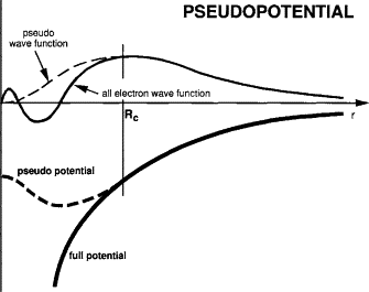
Fig.1: Schematic representation of pseudization procedure for the wave function and the corresponding generating potential.

Important Ideas and Observations:

Several schemes exist for constructing pseudopotentials. In our work, I focused on the Projector Augmented Wave (PAW) method[2-4], one of the most widely used and accurate approaches.

The computational cost of a DFT calculation can be broadly estimated as: Cost ~ \(N_{\rm SCF} \times C_{\rm step}\) ,
where
– \(N_{\rm SCF}\) is the number of self-consistent field iterations,
– \(C_{\rm step}\) is the cost per SCF step.
The latter is dominated by the diagonalization of the Hamiltonian matrix, which scales approximately as \(C_{\rm step} ∝ N_{\rm PW}\log N_{\rm PW}\) with \(N_{\rm PW}\) being the number of plane waves in the basis, which is usually determined by the cutoff energy is DFT setting. Thus, softer pseudopotentials (which require fewer plane waves) lead to cheaper calculations, but often at the expense of accuracy and transferability i.e. ability of the single element PAW dataset to be able to accurately simulate physical properties across various bonding environments.

Some important trade-offs:
– Norm-conserving pseudopotentials: high accuracy, but computationally demanding.
– Ultrasoft (or smooth) pseudopotentials: computationally efficient, but sometimes less accurate and less transferable.
– PAW method: attempts to combine the best of both by reconstructing AE wavefunctions from smooth pseudowavefunctions with the help of augmentation functions.

In this study, we optimize the degrees of freedom in the PAW-type pseudopotential, as detailed in the following chapter, to achieve accuracy comparable to norm-conserving methods while preserving smoothness.

Optimization Idea:

To illustrate: suppose we consider silicon (Si). In our approach, we constructed the projectors for augmentation of valence electrons using s, p, d orbital solution of the atomic Schrödinger equation. According to the theory of PAW method[2], the local (zero) potential operating on the orbital inside the augmentation radius \(r_c\) does not affect the value of physical observables. It is therefore an arbitrary degree of freedom[4], which we can aim to optimize. This zero potential is usually made smooth to improve SCF convergence. However, the potential affects physical observables if the wavefunction includes higher-order angular momentum components because the projectors are not complete. This actually happens if the system is a multi-atom system, i.e. not the ideal single atom system, and the f-orbital element is primarily mixed into the valence orbital. We optimize the zero potential to be accurate for the f-orbital:

\(\left[ -\frac{1}{2}\frac{d^2}{dr^2} + \frac{l(l+1)}{2r^2} + V^{\rm PS} (r)\right] u_l^{PS}(r) = E u_l^{PS}(r),\)

\(V^{PS}(r) = E -\frac{l}{r^2}+ \frac{l}{r}\frac{a'(r)}{a(r)} + \frac{1}{2}\frac{a”(r)}{a(r)}, \) (★)

\(u_l^{PS}(r) = r^la(r),\)

where the local potential is defined as \( V_{\rm PS}(r) = V_{\rm H}(r) + V{\rm xc}(r) + V_0(r) \). For the reference energy \(E\), we used 0 eV. For the reference f-orbital, we rather use an optimized orbital rather than true (all-electron) one so that the resulting zero potential becomes transferable and smooth.

We chose to perform optimization while imposing two key physical constraints on the wave function pseudization procedure:

Norm conservation condition to reproduce scattering property of f-orbital: \( \int_0^{r_c} |\phi_l(r)|^2 r^2 dr = \int_0^{r_c} |\tilde{\phi}_l(r)|^2 r^2 dr \),
Log-derivative matching at \(r = r_c\): \(\frac{1}{\phi_l(r)} \frac{\partial \phi_l(r)}{\partial r} = \frac{1}{\tilde{\phi}_l(r)} \frac{\partial \tilde{\phi}_l(r)}{\partial r}\)

where \(\phi_l\) and \(\tilde{\phi}_l\) are pseudowavefunction and all-electron wavefunction, respectively.

This procedure was implemented on GPAW and it proceeds as follows:

First, perform a smooth pseudization of the AE wavefunction.
Next, enforce the above constraints by fixing value at two points (the location of these points in (0, \(r_c\)) can be treated as free parameters).
Finally, with some additional interpolation points and using cubic splines to smoothly connect all the points to make the final pseudo wavefunction. This wave function then defines \(V_{\rm PS}\) and \(V_0\) as defined above in eqn. (★) .

Implementing Optimization Procedure:

In addition to the free parameters (such as the choice of fixed points for pseudization), the augmentation radius must also be updated. Adding new f-orbitals can enlarge or reduce the augmentation region to satisfy orthogonality constraints with existing orbitals.

To guide the optimization, I defined the following objective functions that form a multi-objective cost function in Optuna:

Convergence to Ground State Energy (\(E_{\rm gs}\)): minimize \(E_{\rm cut}\) such that \( |E_{\rm cut} – E_{\rm ref}| < 1 \) meV. The “ref” cutoff is often chosen as some large value such as 1000 or 1200 eV.
Convergence to Band Gap, (Δbg): minimize \(E_{\rm cut}\) such that \( |E_{\rm cut} – E_{\rm ref}| < 1 \) meV
Number of SCF steps(N): minimize (\(\frac{1}{N} E_{\rm cuts}∑N_{\rm scf} \) ) while \( |E_{\rm cut} – E_{\rm ref}| < 1 \) meV. This average is calculated using the SCF steps from \(E_{\rm cut}\) values that did not meet the convergence criteria.”
Norm of Gradient zero potential: minimize \(\int_0^{r_c} |\nabla V^{\rm PS}\)

For multi-objective optimization, we used Optuna with only ~5 trials per element (each run taking 12–20 hours and significant memory). There are two available samplers, NSGA-II and TPE. In this study, we used the NSGA-II sampler.

This optimization workflow is briefly summarized in the flowchart below: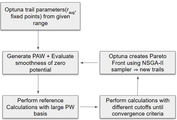

Fig2: The optimization workflow of zero potential of PAW.

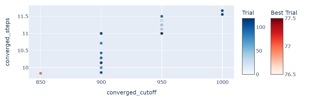
Fig.3: Pareto-front chart obtained while performing optimization for Mg. Every point on the plot indicates a PAW dataset generated using trial parameters suggested by Optuna. In the plot, outputs are projected onto space spanned by two objectives (\(N_{\rm SCF}, E_{\rm cut}\) )

Results and Conclusions:

We performed all the validation calculations using GPAW[5] along with ASE[6]. To benchmark the approach, we compared three PAW datasets:1.Smooth reference PAW (no norm conservation), 2.Additional f-orbital PAW (with norm conservation but no optimization), 3.Optimized PAW (with multi-objective optimization).For non-metallic elements(Si) (\(\delta_{\rm bg}\)>0), simply introducing the f-orbital norm conservation already improved efficiency, visible from the reduced Ecut for GS convergence. Further optimization marginally refined this. In contrast, metallic elements (Fe, Mg) proved more difficult to optimize. Even after optimization, their computational performance was slightly worse than the reference smooth PAWs. (Fe, Mg) (Fig.4)

ref: smooth PAW datasets without norm conservation on any orbital provided with the GPAW code at https://gpaw.readthedocs.io/setups/setups.html .

scattering-F: custom generated PAW with additional norm conservation on f-orbital.

optim-scattering-F: custom generated PAW with additional norm conservation on F-orbital after optimisation.

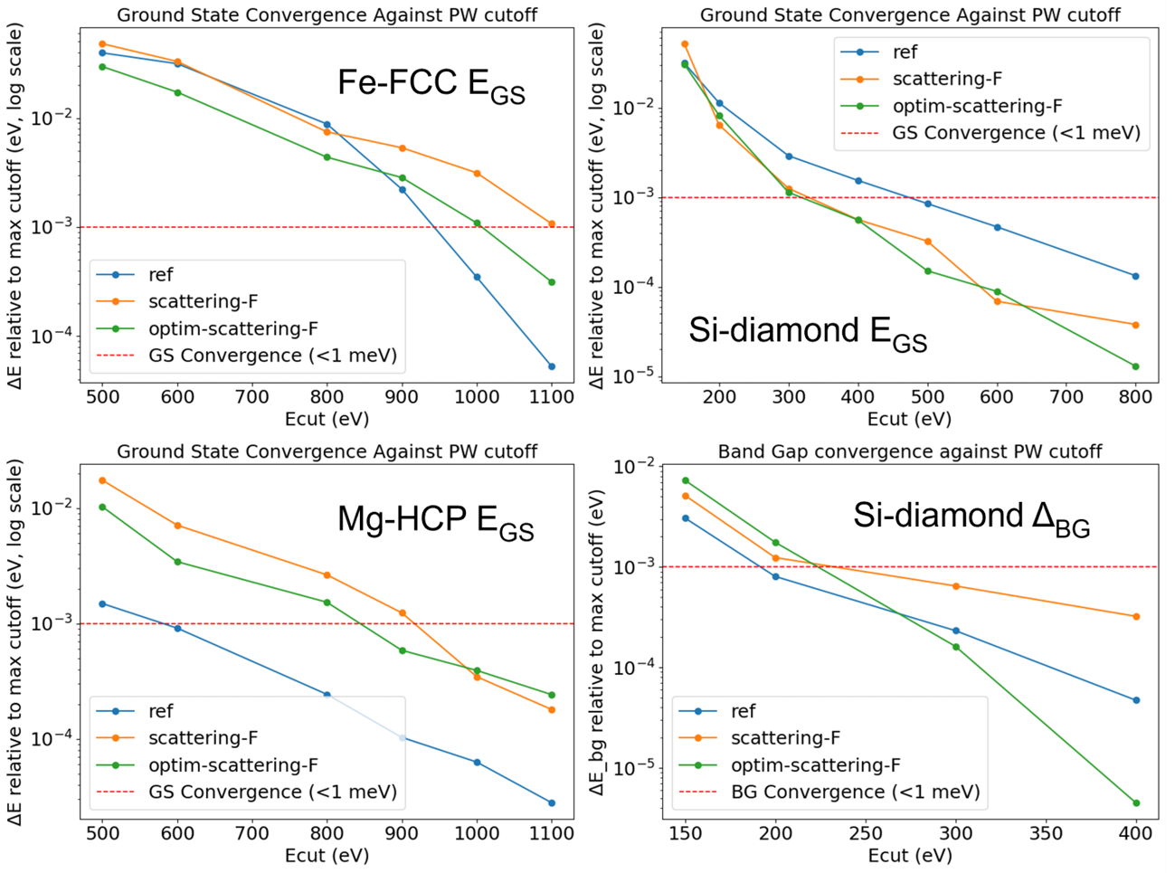
Fig.4 : Optimization results for Mg, Fe, Si: (top-left, top-right, bottom-left) GS convergence for Fe FCC(Face Centered Cubic), Si-diamond and Mg-HCP(Hexagonal Closed Packing) respectively with above defined 3 PAW datasets. (bottom-right) \(\delta_{\rm bg}\) convergence for Si using the same PAWs.

To build some intuition, we also plotted the zero potential for Si and Mg before and after optimization. As shown in Fig. 5, optimization reduces the number of nodes in \(V_0(r)\) while the pseudization of the wave function for f-orbital respects the norm and log-derivative constraints.

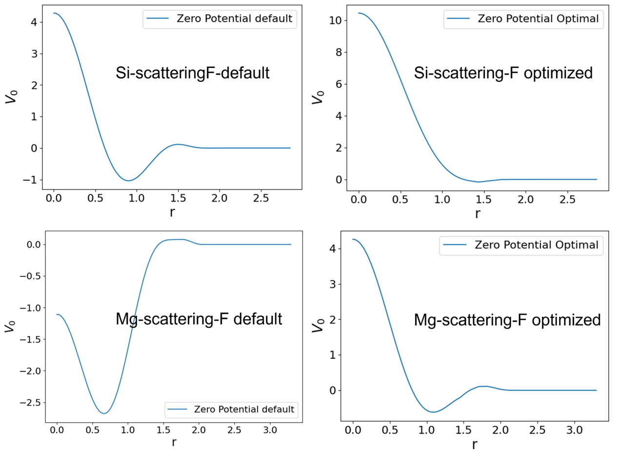
Fig.5 : Optimized vs Default zero potential for Mg and Si.

The benefit is more evident in heteroatomic systems such as FeSi, where Fe and Si have very different valence orbitals. Without optimization, the Fe and Si PAWs generated with additional f-orbital when coupled together fail to converge even after 100 SCF steps. Whereas after optimization, convergence is achieved reliably in terms of all the optimization objectives \( E_{\rm GS}\), \(N_{rm SCF}\), \(\delta_{\rm bg} \) . Similarly, for Mg2Si although GS convergence is not better than reference dataset (optimised for smoothness), faster convergence in terms of band gap(\(\delta_{\rm bg}\)) can be observed from Fig. 6.

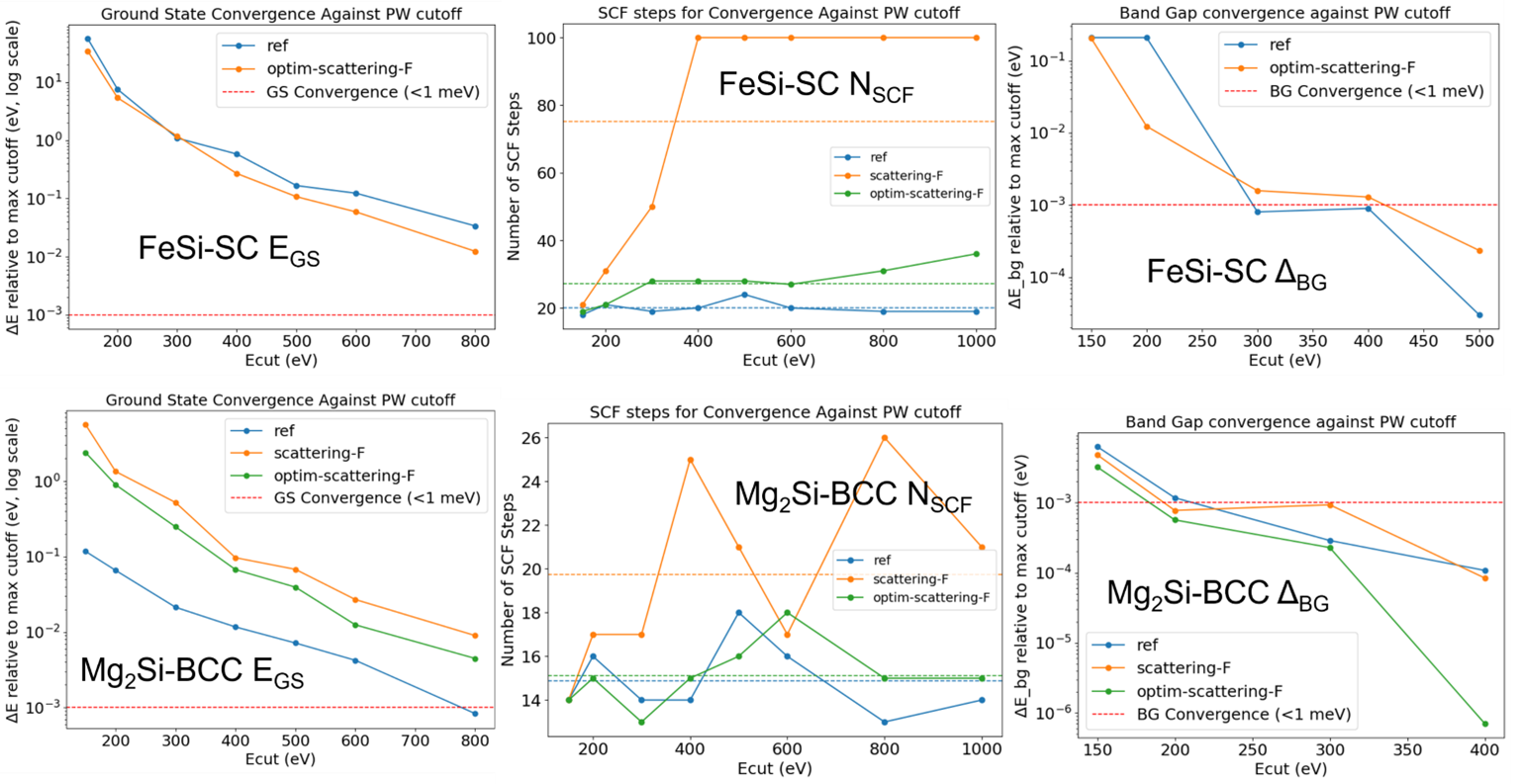
Fig.6: Validations for Mg2Si, FeSi: (top-left, top-middle, top-right) EGS convergence, NSCF convergence and Δbg convergence for FeSi- SC (Simple Cubic B20-type structure). (bottom-left, bottom-middle, bottom-right) similar convergence tests for Mg2Si-BCC (Body Centered Cubic). The dashed lines in NSCF plots represent the average number of steps for convergence across different \(E_{\rm cut}\).

Comparisons with all-electron FP-LAPW(Full Potential Linearised Augmented Plane Wave) calculations also confirm the accuracy of the optimized PAWs:

Mg₂Si: Optimized PAW gives a band gap of 0.207 eV, close to the LAPW value (0.21–0.23 eV)[7], while the reference PAW gives only 0.191 eV.
FeSi: Optimized and reference PAWs yield 0.170 eV and 0.175 eV respectively, compared to ~0.130 eV[8] from LAPW. Note: All electron calculations also perform poorly in case of strongly correlated electronic systems like FeSi without additional corrections.

Finally, to check that optimization does not overfit the chosen objectives, I performed Equation of State (EOS) calculations for Si and Mg. The bulk modulus from optimized and reference PAWs matched almost perfectly. The equilibrium lattice constant was also consistent with all-electron results obtained using Wien2k parameters, except for a slight deviation in Mg (Fig.7).

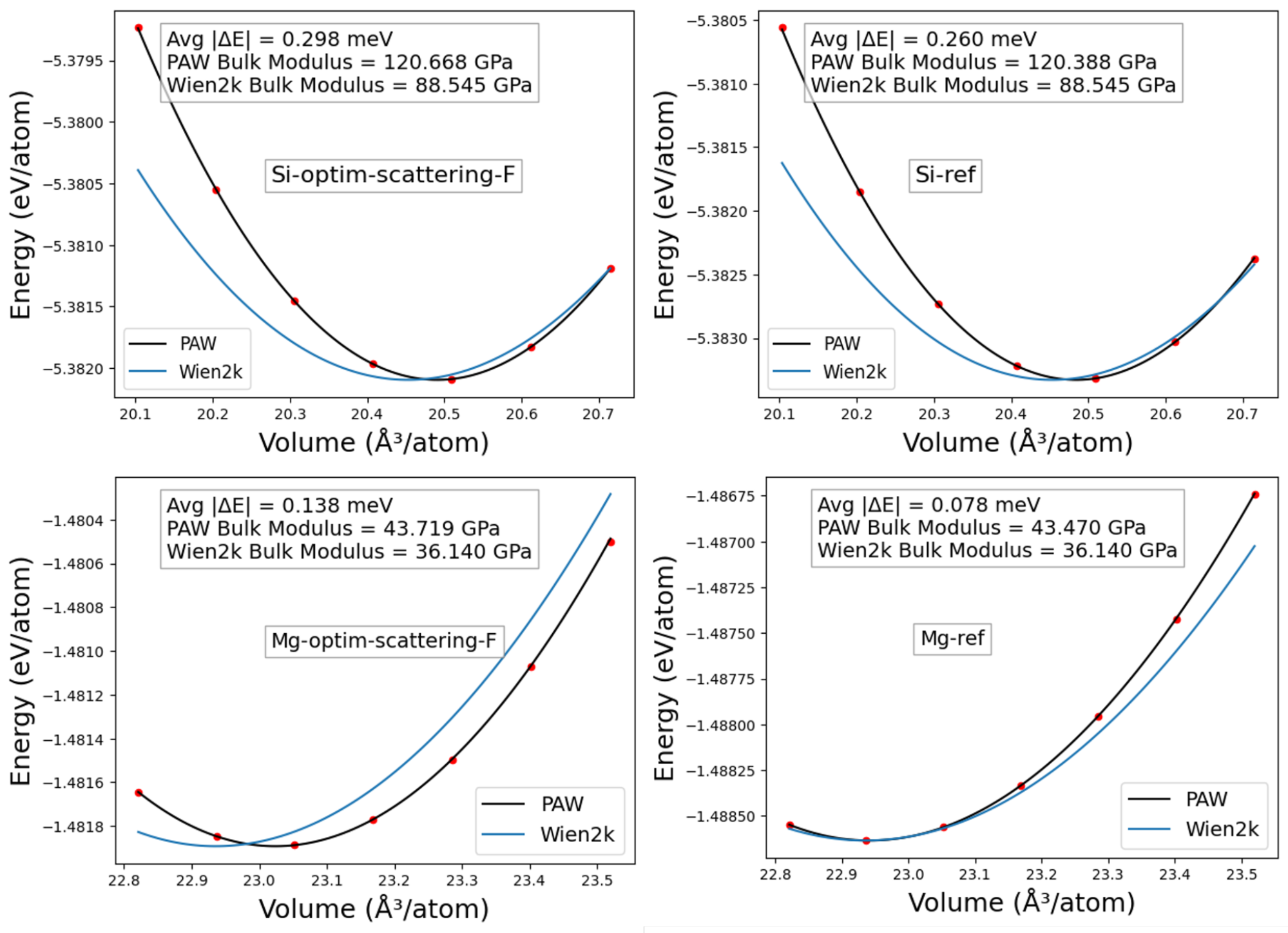
Fig.7: EOS plots for Mg and Si comparing equilibrium lattice constant and Bulk Modulus with all electron calculations(Wien2k) with reference and optimized PAW.

In conclusion, the proposed method appears capable of generating more transferable PAW datasets without a significant increase in computational cost as observed from band gap predictions and convergence rate in FeSi and Mg2Si. However,

Much broader validation is still required across different classes of elements to fully establish the robustness of the procedure.
In addition, more efficient optimization strategies could be implemented to allow a larger number of Optuna trials to reach the recommended trial limit for the samplers used.
Finally, the development of additional constraint conditions may be necessary for metallic elements, which tend to converge more slowly during optimization.

For further improvement, there is room for refinement in the definition of the constraints.

References:

A. Filippetti and G.B. Bachelet, Pseudopotential Method, Encyclopedia of Condensed Matter Physics, Elsevier (2005)
P. E. Blöchl, Projector augmented-wave method, Phys. Rev. B 50, 17953 (1994).
G. Kresse and D. Joubert, From ultrasoft pseudopotentials to the projector augmented-wave method, Phys. Rev. B 59, 1758 (1999).
J. J. Mortensen, L. B. Hansen, and K. W. Jacobsen, Real-space grid implementation of the projector augmented wave method, Phys. Rev. B 71, 035109 (2005).
GPAW: An open Python package for electronic-structure calculations. Available at: https://gitlab.com/gpaw/gpaw.
A. H. Larsen et al., The atomic simulation environment, a Python library for working with atoms, J. Phys.: Condens. Matter 29, 273002 (2017).
P. Boulet, M. J. Verstraete, J.P. Crocombette, M. Briki, and M.C. Record, Electronic properties of the Mg2Si thermoelectric material investigated by linear-response density-functional theory, J. Phys. Chem. C 116, 21791 (2012).
S. Khmelevskyi, G. Kresse, and P. Mohn, Correlated excited states in the narrow band gap semiconductor FeSi and antiferromagnetic screening of local spin moments, Phys. Rev. B 72, 064510 (2005).