Blog
This post is contributed by Pragyan Shrestha, who was an intern at PFN.
I am Pragyan Shrestha, a first year graduate student at University of Tsukuba. My research topic is 3D reconstruction from 2D X-ray images. In this internship, we worked on reconstructing dynamic CT volumes using implicit neural representation and differentiable X-ray transform.
Introduction
Four Dimensional CT
Computed Tomography (CT) is a well established technique to reconstruct the interior structure of an object from its projections. An X-ray generating source in a CT scanner emits the ray towards the region of interest (ROI) of the patient body and the detectors capture the projections. The source and the detector move around the object to scan the trans-axial plane in a single revolution. The image of the plane is reconstructed using the acquired projections.
An example of CT reconstruction. Cited from: https://en.wikipedia.org/wiki/Tomographic_reconstruction
The observed values are called “raw data,” which are either 1D (parallel beam setting) or 2D (cone beam setting). In the parallel beam setting, generally a single 2D slice is reconstructed from raw data collected at multiple angles, whereas a 3D volume is directly reconstructed from multiple 2D projection images in the cone beam setting.
A key factor to assure in taking CT scans is suppression of artifacts. Motion artifact is one of them and is often problematic when we take CT scans that include moving organs, such as the lungs and heart. The motion of such organs during a scan results in blurriness and double images in the reconstructed CT volumes. An apparent solution would then be to increase the collimation (scan region) and acquisition rate. Indeed there exist 256-slice CT scanners that can operate at much higher rates enabling 4D reconstructions using continuous application of 3D technique. However, not all healthcare institutes possess such powerful devices. The standard way to do cardiac CT (CT scan of heart) is by gating methods[1]. The periodic motion of heart or lungs is exploited to rebin the acquired projections into phases (usually up to 10). 4D reconstruction algorithms can then be applied to reconstruct each phase. This requires external gating signals such as ECG or phase extraction methods[2] if the projection image is 2D (cone beam setting). Phase estimation errors along with irregularity in motion can still introduce artifacts. To overcome these problems, we propose a method that does not rely on phases nor assume completely periodic motion.
Applying implicit neural representation to 4DCT
An implicit neural function maps spatial coordinates to the desired output at the query point. This output can be occupancy values, signed distance function, attenuation constant, or any meta information. NeRF[3] and its variants map the 6 dimensional input (spatial coordinates and view direction) to the RGB and opacity values. Along with differentiable rendering, it enables learning a resolution-independent radiance field with only 2D supervision. It can also save memory consumption compared with conventional ways such as voxel or mesh representation [4].
Reed AW, et al.[5] proposed a 4DCT reconstruction method based on implicit neural representation (INR). They disentangle time and space by using template volume and warp volume. They were able to reconstruct dynamic volumes of thorax with satisfactory PSNR. However, the geometry used was parallel beam setting, which today is used in less available synchrotron scanners. Also, their sampling scheme is grid based, thus limiting the resolution of the reconstructed volume.
In this research, we propose to extend their approach by focusing on cone beam setting rather than parallel beam one, aiming at the practical use of the reconstruction method in the future, and by randomly sampling rays from all the pixel coordinates in the detector rather than grid sampling.
Proposed method
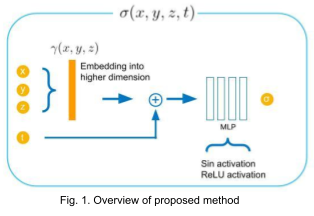
We propose to directly regress attenuation constant \( \sigma(x,y,z,t) \) using 3D spatial coordinates and time (Fig. 1). This allows us to generate reconstructed voxel volume at an arbitrary time by sampling voxel grid locations and concatenating the given time variable with the sampled points. For reconstructing high frequency details, we map the spatial coordinates into higher dimensional embeddings (256 dimensions) using Gaussian random Fourier features with variance of 1 [6].
One of the major challenges that we encountered was to discover how to integrate the time variable into the network architecture. We cover 2 variants that we tried in the experiments section.
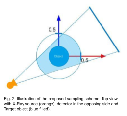
The coordinates are normalized such that the volume boundaries and time lie between [-0.5, 0.5] and [0, 1] respectively. During the training, the points are sampled such that each of them lies within a cylindrical region as illustrated in Fig. 2. For the rendering of projection images, we discretize the X-ray transform using Riemann summation and apply the following equation to obtain the projection value from attenuations sampled from a ray.
\[ R(\boldsymbol \alpha, \boldsymbol s) = \int_{L}^{} f(\boldsymbol x) d \boldsymbol x \approx \sum_{i=0}^{N_{\mathrm{rays}}-1} \sigma((1-\frac{i}{N_{\mathrm{rays}}}) \boldsymbol x_{\mathrm{entry}} + (\frac{i}{N_{\mathrm{rays}}}) \boldsymbol x_{\mathrm{exit}}) \delta_{i} \]
Here, the function \( R \) maps the X-ray source position and ray direction into the projection value. It is modeled as the line integral of the attenuation function \( f(x,y,z) \), which is what we want to reconstruct. The equation in the R.H.S is the discretized form of the line integral where \( \sigma \) is obtained by querying the INR and \( \delta_i \) is the distance between \( i^{\mathrm{th}} \) and \( (i+1)^{\mathrm{th}} \) sample points.
Experiments
Dataset
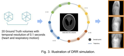
We use the XCAT[7] phantom to produce dynamic human body volumes with respiratory and cardiac motion. The framework TIGRE[8] is used to produce digitally reconstructed radiographs (DRRs) from dynamic or static volumes. As shown in Fig. 3. 20 ground truth volumes with temporal resolution of 0.1 seconds between each consecutive volume were generated with the XCAT phantom. For the static volume dataset, we generate 100 projections around 360 degrees with the first volume. For the dynamic volume dataset, we generate 5 projections from each volume. The acquisition geometry for each volume is adjusted such that we get 100 projections with 360 degrees coverage in total. The images in the right most region of Fig. 3. are some examples of the projection images (DRRs).
Reconstruction results
First, we compare the reconstruction of a static volume (without time input) with conventional 3D methods (SART[9] and FDK[10]). Fig. 4. shows the reconstructed axial slices with each method. Fig. 5. shows the quantitative comparisons in terms of PSNR and SSIM for each reconstructed slice image.
Fig. 4. Reconstructed axial slice images
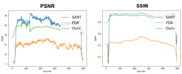
Fig. 5. Quantitative comparison of the reconstruction. The metrics are calculated over each slice image individually.
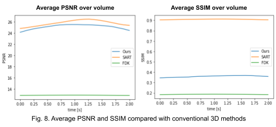
Second, we reconstruct the dynamic volume and compare it with the 3D methods. Fig. 6. shows the coronal slice of the human body with respiratory motion and heart motion with our method. Fig. 7. shows the coronal slice of the human body reconstructed with 3D methods (by assuming all the projection images are taken from a static volume). Fig. 8 shows the average PSNR and average SSIM, which is the average over slices in a volume, calculated over all 20 corresponding volumes. For 3D methods, the same volume is used as the target for all volumes.
Fig. 6. Coronal slices of the reconstructed dynamic volume with our method.
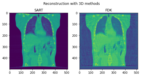
Fig. 7. Coronal slices of the reconstructed volumes with 3D methods.
Encoding variants
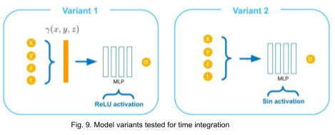
We try incorporating the time variable in two other ways as illustrated in Fig. 9. In variant 1, the time variable is encoded along with spatial coordinates using original positional encoding (12 frequencies for each coordinate) used in NeRF. In variant 2, the input to the MLP is not encoded explicitly, instead sine activations are used in all layers excluding the output [11].
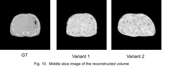
Fig. 10. shows the middle slice image of the reconstruction. We stopped the training at an early stage because the networks got stuck in local minima.
Discussions
The result of reconstruction for static volume is not up to par with the conventional methods. As shown in Fig. 4, the PSNR and SSIM of our method were close to those of SART, and beat those of FDK by a large margin. However, the actual reconstruction in Fig. 3. shows that the reconstructed volume with our proposed method is missing high-frequency information, suggesting that the images produced by FDK are still a better choice for diagnosis compared to ours. Such a situation may be overcome by employing a different loss function, network architecture or aggregation function. This is left for future experimentation and research.
Unlike the conventional methods used to reconstruct 3D CT from raw observations, which create the double image motion artifacts for heart and lungs, our method can successfully reconstruct them without such artifacts in a dynamic CT scan. Despite such achievement, our method could not achieve reconstruction of the high-frequency information. As shown in Fig. 8, the PSNR and SSIM of our method were lower than those of SART. In order to put our proposed method to practical use, we have to seek alterations that can preserve high-frequency information in the reconstruction.
Further improvements may be achieved by introducing hierarchical resolution sampling (i.e., training low resolution images then gradually increasing the resolution), adding perturbations in the sampled points, or modifying the rendering equation to match the forward projection model (such as Siddon ray marching) used in the conventional methods.
Conclusion
Although the image quality has room for improvement, we have demonstrated the possibility of using implicit neural representation for reconstructing dynamic CT volumes using only the projection images and the geometry.
Acknowledgments
I would like to thank my mentors Hirano-san and Deniz-san for giving me very informative and clear advice. I learned a lot from them as well as other internship fellows. It was a great experience for me to have participated in the program.
References
[1] Desjardins, Benoit, and Ella A. Kazerooni. “ECG-Gated Cardiac CT.” American Journal of Roentgenology, vol. 182, no. 4, American Roentgen Ray Society, Apr. 2004, pp. 993–1010.
[2] Zijp, Lambert, et al. “Extraction of the Respiratory Signal from Sequential Thorax Cone-Beam X-Ray Images.” ICCR, Jan. 2004
[3] Mildenhall, Ben, et al. “NeRF: Representing Scenes as Neural Radiance Fields for View Synthesis.” arXiv [cs.CV], 19 Mar. 2020, http://arxiv.org/abs/2003.08934. arXiv.
[4] Kato, Hiroharu, et al. “Differentiable rendering: A survey.” arXiv [cs.CV], 22 June 2020, http://arxiv.org/abs/2006.12057. arXiv.
[5] Reed, Albert W., et al. “Dynamic CT Reconstruction from Limited Views with Implicit Neural Representations and Parametric Motion Fields.” arXiv [eess.IV], 23 Apr. 2021, http://arxiv.org/abs/2104.11745. arXiv.
[6] Tancik, Matthew, et al. “Fourier Features Let Networks Learn High Frequency Functions in Low Dimensional Domains.” arXiv [cs.CV], 18 June 2020, http://arxiv.org/abs/2006.10739. arXiv.
[7] Segars, W. P., et al. “4D XCAT Phantom for Multimodality Imaging Research.” Medical Physics, vol. 37, no. 9, Sept. 2010, pp. 4902–15.
[8] Biguri, Ander, et al. “TIGRE: A MATLAB-GPU Toolbox for CBCT Image Reconstruction.” Biomedical Physics & Engineering Express, vol. 2, no. 5, IOP Publishing, Sept. 2016, p. 055010.
[9] Andersen, A. H., and A. C. Kak. “Simultaneous Algebraic Reconstruction Technique (SART): A Superior Implementation of the ART Algorithm.” Ultrasonic Imaging, vol. 6, no. 1, Jan. 1984, pp. 81–94.
[10] Feldkamp, L. A., et al. “Practical Cone-Beam Algorithm.” JOSA A, vol. 1, no. 6, Optical Society of America, June 1984, pp. 612–19.
[11] Sitzmann, Vincent, et al. “Implicit Neural Representations with Periodic Activation Functions.” arXiv [cs.CV], 17 June 2020, http://arxiv.org/abs/2006.09661. arXiv.
