This post is a contribution by Zongyao Li, who was an intern at PFN.

I am Zongyao Li, a Ph. D. student at Graduate School of Information Science of Technology, Hokkaido University. I participated in the PFN summer internship program in 2022. During the internship, I did research on test-time adaptation for brain tumor segmentation with cross-institutional MRI. In this article, I would like to share our ideas and results in the research.

Introduction

Mismatch between distributions of training and test data, which is typically referred to as domain shift, has been a long-term problem in the field of machine learning. The domain shifts between training and test data deteriorate the performance of machine learning models considerably. In the field of medical imaging, the above problem is quite common, and the domain shifts may arise due to different scanners and imaging protocols in different institutions. Figure 1 shows an example of the performance drop in the segmentation task for which we aim to reduce the domain shifts. Because it is extremely difficult and costly to obtain well-annotated medical images, a method that can tackle the domain shifts without using any additional annotations is desired. In this research, we worked on such a problem setting called test-time adaptation.

Test-time adaptation aims to suppress the performance drop on the target-domain test data by performing domain adaptation at test time with only the pre-trained source-domain model. Compared to the general domain adaptation setting, test-time adaptation is much more challenging since the source-domain data is inaccessible at test time. Moreover, the access to the target-domain distribution is also limited to some extent, while the limitation is not strictly defined and varies in different researches. In our research, we dealt with the most challenging setting in which only one test sample is available each time, and the continual test samples are not assumed to belong to the same domain. More concretely, we trained a brain tumor segmentation model with MRI data from one institution and performed test-time adaptation for MRIs from different institutions.

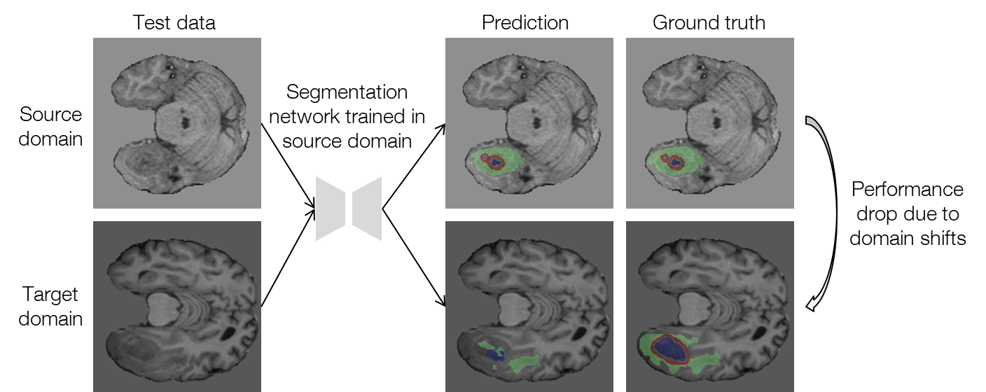
Figure 1. An example of performance drop when applying the source-domain model to the target domain for segmenting brain tumors with MRI (data provided by FeTS Challenge 2022 [1-3]).

Related work

Related work on test-time adaptation typically used an unsupervised or self-supervised regularization term to finetune the pre-trained source-domain model or part of the model. For example, entropy minimization, which is a common regularization strategy for training with unlabeled data, has been applied for test-time adaptation by training only the batch normalization layers to minimize the prediction entropy of the test samples [4]. Sun, Yu, et al. [5] introduced an auxiliary task of predicting the rotation angle of a rotated input into the training of the source-domain model and adapted the model at test time with the self-supervised task. In the work [6], another self-supervised learning strategy, contrastive learning, was used to finetune the source-domain model with target-domain images along with pseudo labeling. In particular, the authors also proposed methods that focus on medical imaging tasks. Li, Haoliang, et al. [7] trained the model to learn the source-domain prior information of semantic shapes, which is invariant across domains, and finetuned only the batch normalization layers at test time with consistency regularization. Similarly, another method [8] also shaped the source-domain priors of segmentation by training an additional denoising autoencoder to correct distorted segmentations, and at test time, a shallow CNN was trained to transform the test sample to reduce the domain shifts with the regularization from the autoencoder. It is worth noting that both methods for medical imaging [7] and [8] worked on the basis of consistent segmentation priors, which always exist in organ segmentation but may not be available in tumor segmentation since tumors have much wider varieties of shape, size, and position than organs. In other words, we still lack a test-time adaptation method that works satisfactorily for tumor segmentation.

Test-time adaptation with feature statistics alignment

To suppress the performance drop of brain tumor segmentation with cross-institutional MRI, we propose a test-time adaptation method with feature statistics alignment. Figure 2 illustrates the motivation of our method. To tackle the domain shifts, we aim to align the feature distributions between the whole training set and the test sample. Feature distribution alignment is considered a generally effective strategy for solving domain adaptation problems. However, in our research, the source-domain feature distribution is unseen since the data is inaccessible, which makes the previous feature alignment methods inapplicable to our research. As an estimation of the source-domain feature distribution, we propose to use the feature statistics (i.e., running mean and running standard deviation) stored in the batch normalization (BN) layers of the pre-trained model and assume that the features are normally distributed as the statistics characterize. Similarly, feeding the test sample into the pre-trained model, the feature distribution of the test sample is estimated as the normal distribution characterized by the mean and standard deviation (std) of the features. Then, we can align the feature distributions by minimizing the Kullback–Leibler (KL) divergence between the normal distributions. The loss function of our method is defined as follows: \[L=\frac{1}{B}\sum_{b=1}^{B}\sum_{c=1}^{C_b}\rm{KLD}\left(\mathcal{N}\left(\mu_{b,c}, \sigma_{b,c}^2\right), \mathcal{N}\left(\bar{\mu}_{b,c}, \bar{\sigma}_{b,c}^2\right)\right)\tag{1}\]
where \(B\) is the number of the BN layers, \(C_b\) is the number of channels at the bth BN layer, \(\rm{KLD}(,)\) and \(\mathcal{N}(,)\) denote the KL divergence and the normal distribution, \(\mu_{b,c}\) and \(\sigma_{b,c}\) denote the mean and std of the test sample features at the cth channel of the bth BN layer, and \(\bar{\mu}_{b,c}\) and \(\bar{\sigma}_{b,c}\) denote those of the running statistics of the training data. To minimize the loss of the statistics differences, we use two different adaptation methods described in the following sections. 

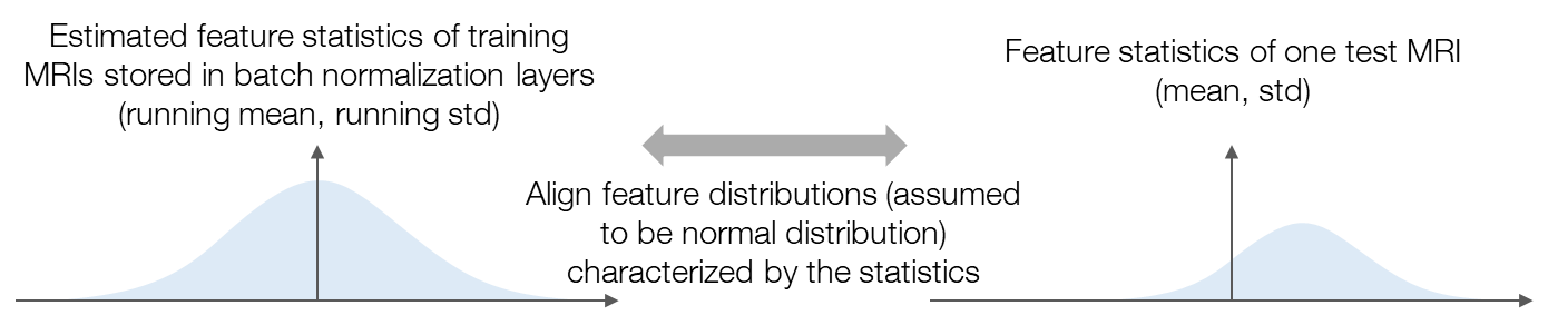
Figure 2. An illustration of the motivation of the proposed method. We assume that the features are normally distributed and align the feature distributions characterized by the feature statistics.

Normalizer adaptation

Inspired by the previous work [8], we first tried training a normalizer network, which transforms the input MRI before segmentation, to consequently adapt the feature distributions. Here, the normalizer network is a shallow CNN with a small receptive field and can therefore only perform simple intensity transformations but not change any structures. The procedure is composed of a training stage and a test stage as shown in Figure 3. In the training stage, we train a normalizer network together with the segmentation network in the same manner as general supervised learning. The input data are fed into the normalizer first and then segmented by the segmentation network, and the two networks are updated together. In the test stage, we perform the test-time adaptation by training the normalizer to minimize the loss function (1) while freezing the segmentation network. For each test MRI, we train the normalizer for some iterations with initial weights inheriting from the training stage and choose the normalized MRI at the iteration of the minimal loss for the final prediction.

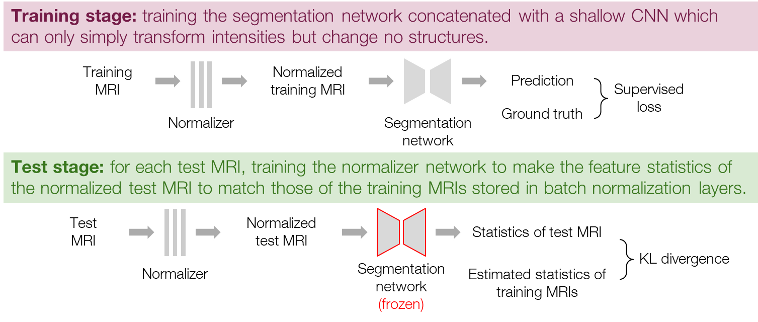
Figure 3. Procedure of the normalizer adaptation.

BN layer adaptation

Since the BN layers with affine parameters can adaptively change feature distributions, we also tried training only the BN layers (i.e. the affine parameters) to directly adapt the feature distributions. The procedure is similar to that of the normalizer adaptation, but the normalizer is removed, as shown in Figure 4. Specifically, the training stage is exactly the same as general supervised learning, and in the test stage, we train the BN layers to minimize the loss in Eq. (1) while freezing the other parameters of the segmentation network. Similarly to the normalizer adaptation, we use the BN parameters at the iteration of the minimal loss for the final prediction. Note that in both the normalizer adaptation and the BN layer adaptation, the BN layers are set to inference mode so that the running statistics are not updated and remain as the statistics of the training data.

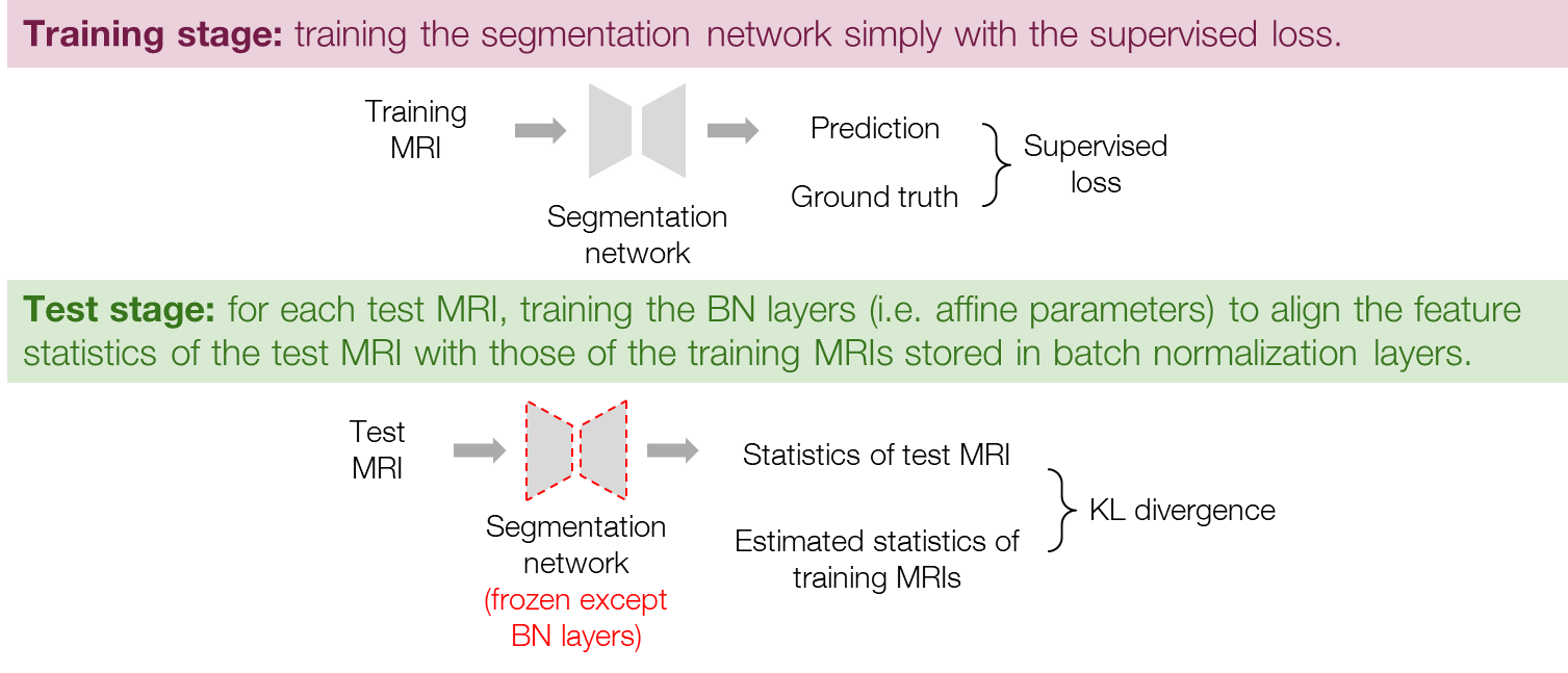
Figure 4. Procedure of the BN layer adaptation.

Experiments

Research data

In the research, we used the data provided by the Federated Tumor Segmentation (FeTS) Challenge 2022 [1-3]. The dataset includes MRI scans of 1251 cases each of which consists of T1, post-contrast T1-weighted (T1Gd), T2-weighted (T2), and T2 Fluid Attenuated Inversion Recovery (T2-FLAIR) modalities. Figure 5 shows an example of 2D slices of the four modalities. Annotations for the brain tumors are composed of the GD-enhancing tumor (ET), the  edematous/invaded tissue (ED), and the necrotic tumor core (NCR). Figure 6 illustrates the three tumor classes. The MRI data are collected from 23 institutions and partitioned by institution. As shown in Figure 7, the two largest partitions 1 and 18 include 511 and 382 cases respectively, and each of the others includes less than 50 cases.

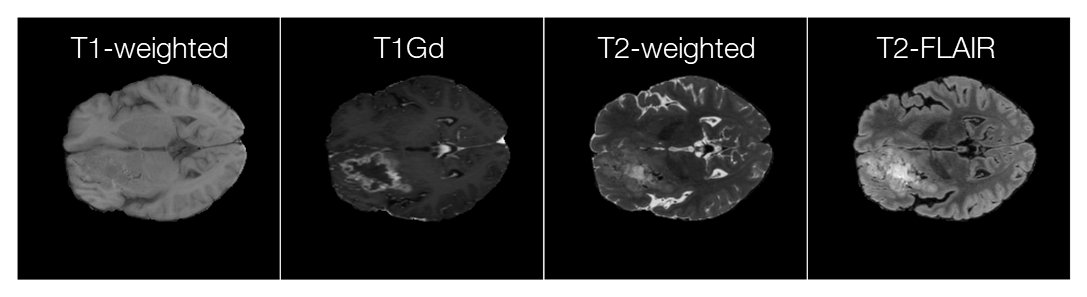
Figure 5. An example of 2D slices of the four MRI modalities (data provided by FeTS Challenge 2022 [1-3]).

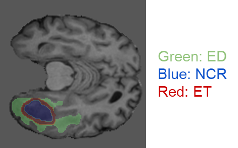
Figure 6. An example MRI slice with its annotations illustrating the brain tumor classes (data provided by FeTS Challenge 2022 [1-3]).

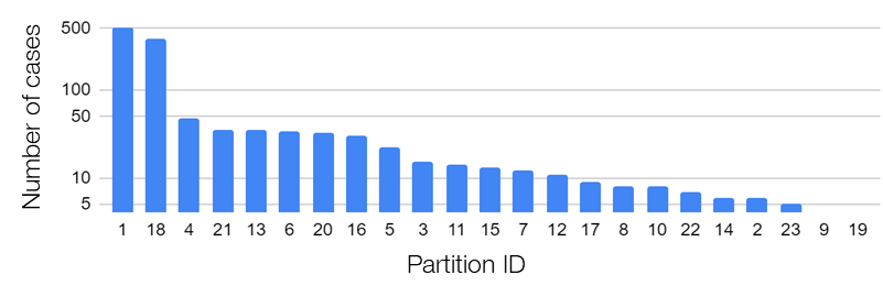
Figure 7. Data distribution across 23 institutions/partitions of the FeTS Challenge 2022 dataset.

Implementation details

We used the dynamic U-Net [9] as the baseline segmentation model. We trained the model for 255 epochs using a RAdam optimizer with an initial learning rate of \(1.0\times10^{-3}\) and a batch size of 4. The normalizer network consists of three convolutional layers with kernel size 3, stride 1, and the number of filters 16 except the last layer. We trained one normalizer for each modality respectively, and the four modalities were concatenated as 4-channel inputs to the segmentation network. In the test-time adaptation, the normalizer and the BN layers were trained with an SGD or Adam optimizer with a learning rate of \(1.0\times10^{-3}\) or \(5.0\times10^{-3}\) for 20 or 50 iterations. The training hyperparameters changed along with different adaptation methods and scenarios. For the BN layer adaptation, we trained only the BN layers of the input block and the downsample block of the baseline model.

Experimental results

We used respectively partition 1 and partition 18 as the source domain to train the segmentation model and evaluated our test-time adaptation method on all the other partitions with the Dice coefficient. Specifically, we report the results on partition 18 (if partition 1 is the source domain and vice versa), partition 13 on which both the models trained on partition 1 and partition 18 performed poorly, and all partitions except partitions 1 and 18. Table 1 and Table 2 show the results using partition 1 and partition 18 as the source domain, respectively.

Table 1 confirms improvements by the test-time adaptation for training on partition 1 and testing on partitions 13 and 18. Both the normalizer adaptation and the BN layer adaptation improved the segmentation performance on partitions 13 and 18, especially for the class NCR on partition 13. On all except 1 and 18, the test-time adaptation changed the results little, and the normalizer adaptation even caused slight degradation. As to the results training on partition 18, as shown in Table 2, we can still see considerable improvements on partition 13 and slight changes with both improvement and degradation on all except 1 and 18, which showed the same tendency as the results training on partition 1. However, unlike the improvements on partition 18, the test-time adaptation failed to improve the performance significantly on partition 1, which showed asymmetric relations of the adaptation performance between partition 1 and partition 18.

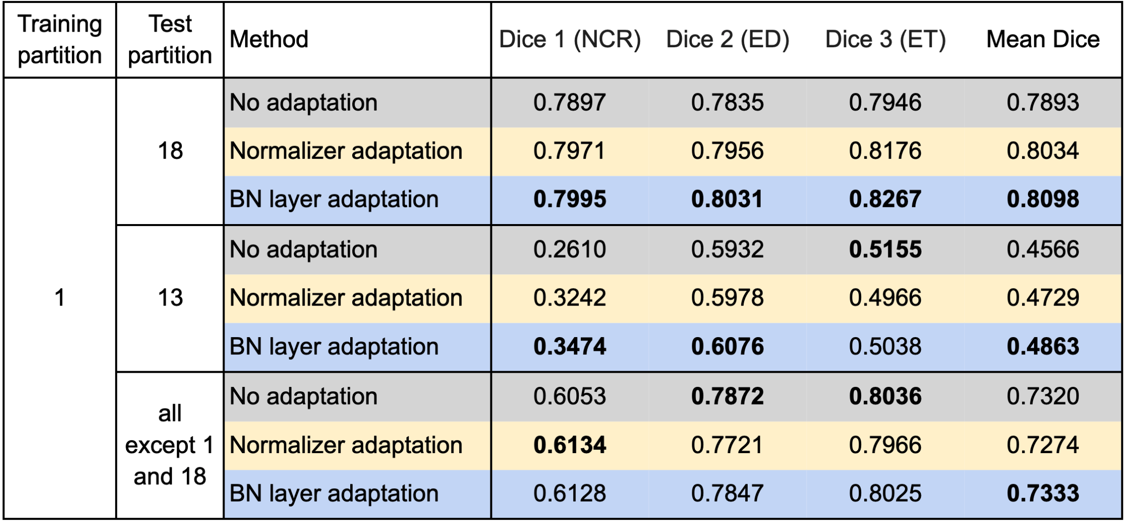
Table 1. Results training on partition 1 and testing on the other partitions.

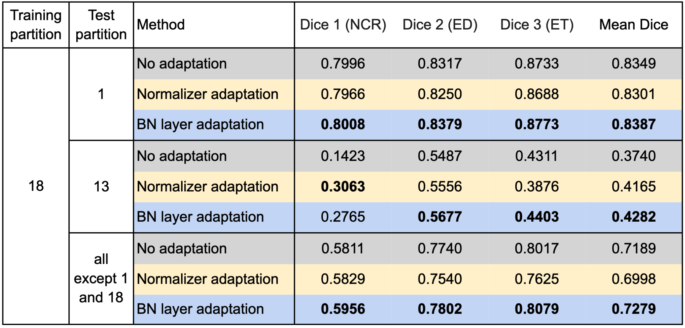
Table 2. Results training on partition 18 and testing on the other partitions.

Analyses

The results in Table 1 and Table 2 verified the effectiveness of the proposed method in some specific scenarios. In the preliminary experiments which are not reported in this article, both the models trained on partition 1 and partition 18 performed worst on partition 13 among all the partitions. Moreover, we can see that the model trained on partition 18 performed fairly well on partition 1 without adaptation, which we think was the reason for no improvement with adaptation. The above observations indicate that the test-time adaptation method is effective for cases with a large performance drop and can hardly work if the performance drop is relatively small. As to the asymmetry between partitions 1 and 18, we think it might be explained by a guess that partition 18 includes a wider variety of sub-domains than partition 1 and partly includes partition 1, which we did not validate.

To explain why the test-time adaptation worked on only part of the partitions, we analyzed the correlation between the difference in feature statistics (i.e. the loss in Eq. (1)) and the mean Dice score without adaptation. Figure 8 shows the analysis results on partition 18 (left) and all except 1 and 18 (right) respectively. We can see a weak negative correlation in the plots, and the correlation coefficients shown above the plots also confirmed the correlation. This weak correlation partly supports our motivation which is to improve the performance by aligning the feature statistics between training and test data, and might also explain the incomplete effectiveness of the proposed method.

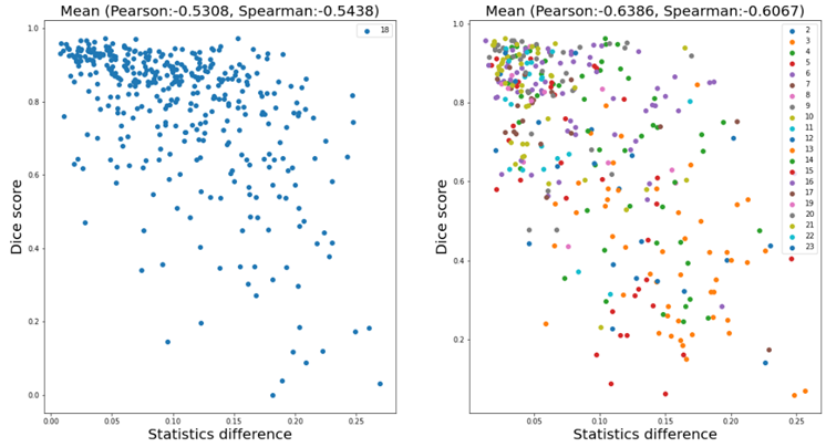
Figure 8. Correlation analysis between the difference of feature statistics and the mean Dice score without adaptation. The model was trained on partition 1. The left plot exhibits the results for samples in partition 18, and the right one for all except 1 and 18.

Conclusion 

In this research, we proposed a test-time adaptation method to suppress the performance drop in brain tumor segmentation due to the domain shifts between cross-institutional MRIs. The proposed method clearly improved the segmentation performance for some cases with a large performance drop, while other cases changed little and some were even degraded. Therefore, the effectiveness of the proposed method was partly confirmed. Moreover, there is a limitation that the optimal hyperparameters (e.g. learning rate, number of iterations) for the test-time adaptation vary in different scenarios, which may make the method less practical since additional annotated data of the target domain would be needed for hyperparameter optimization. The development of robust test-time adaptation methods will be an important direction for future work.

Acknowledgments

I really appreciate my mentors Iwasawa-san and Tokuoka-san, and also Sugawara-san in the medical image team, for their kind help and advice during the internship. Thanks to the abundant computing resources in PFN, I could conduct extensive experiments and try many ideas in the seven weeks. I am grateful for the opportunity of the internship which was a very meaningful experience for me.

References 

[1] S.Pati, U.Baid, M.Zenk, B.Edwards, M.Sheller, G.A.Reina, et al., “The Federated Tumor Segmentation (FeTS) Challenge”, arXiv preprint arXiv:2105.05874 (2021).
[2] G.A.Reina, A.Gruzdev, P.Foley, O.Perepelkina, M.Sharma, I.Davidyuk, et al., “OpenFL: An open-source framework for Federated Learning”, arXiv preprint arXiv: 2105.06413 (2021).
[3] U.Baid, S.Ghodasara, S.Mohan, M.Bilello, E.Calabrese, E.Colak, et.al., “The RSNA-ASNR-MICCAI Brats 2021 Benchmark on Brain Tumor Segmentation and Radiogenomic Classification”, arXiv preprint arXiv: 2107.02314 (2021).
[4] Wang, Dequan, et al. “Tent: Fully Test-Time Adaptation by Entropy Minimization.” International Conference on Learning Representations. 2020.
[5] Sun, Yu, et al. “Test-time training with self-supervision for generalization under distribution shifts.” International conference on machine learning. PMLR, 2020.
[6] Chen, Dian, et al. “Contrastive Test-Time Adaptation.” Proceedings of the IEEE/CVF Conference on Computer Vision and Pattern Recognition. 2022.
[7] Li, Haoliang, et al. “Domain generalization for medical imaging classification with linear-dependency regularization.” Advances in Neural Information Processing Systems 33 (2020): 3118-3129.
[8] Karani, Neerav, et al. “Test-time adaptable neural networks for robust medical image segmentation.” Medical Image Analysis 68 (2021): 101907.
[9] Isensee, Fabian, et al. “Automated design of deep learning methods for biomedical image segmentation.” arXiv preprint arXiv:1904.08128 (2019).