Hello, I am Rawin Assabumrungrat, a student majoring in Robotics at Tohoku University. I have been working at Preferred Networks as an intern and a part-time machine learning researcher in the Quantitative Finance Team with Minami-san and Imos-san to conduct research in deep learning and finance. In this blog, I will summarize what I learned and accomplished during this great research journey.

Background

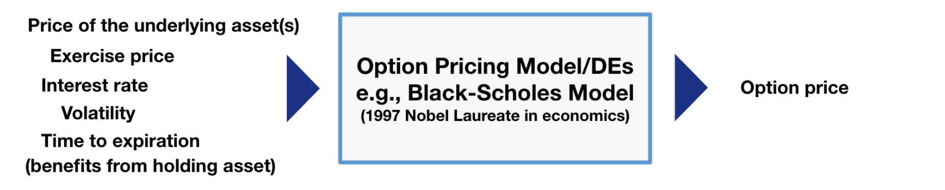
Option pricing is a common problem in the finance world. An option is a contract that gives its holder the right to buy or sell something (called an underlying asset) in the future. A call option gives the holder the right to buy an asset at a specified price, while a put option gives the holder the right to sell an asset at a specified price. An option can be publicly traded in a derivative market or privately as contracts signed between two parties, known as over-the-counter or off-exchange trading. 

However, when the buyer and seller decide to engage in an option transaction, that is, agreeing to grant the option to buy or sell something in the future at a fixed price; a question arises: at what price for the option can both parties mutually agree to? Establishing the “fair value” of the option is key to finding the solution, and it involves finding the expected value of payoffs. When pricing an option, we essentially calculate the expected future gains (or losses) that the option will produce based on multiple economic variables like volatility and then calculate what that value would be worth in terms of today’s value. 

Finding this value is a difficult task that requires knowledge of a variety of market dynamics, economic indicators, and frequently intricate mathematical models. There comes the development of various mathematical models to assist in estimating an option’s price. Many of these models are represented by Stochastic Differential Equations (SDEs). In case of options, their prices are represented by Partial Differential Equations (PDEs) derived from the original SDEs – for example, the famous Black-Scholes model and the Heston model. The equation describes how an option’s price changes over time and with changes in the underlying asset’s price, along with other factors, under certain assumptions. We recommend reading these materials if you are interested: [Link1], [Link2].

To obtain an estimated option price, solving its associated PDE is required. In some cases, an analytic form of the solution exists. However, in most cases, it needs a numerical method, hereby denoted as a “traditional method,” to find the numerical solution on a specific region. However, in case an option has numerous underlying assets, the dimension of PDE is high; the “curse of dimensionality” has made it extremely challenging to solve the PDE. In other words, using the traditional methods, computational time increases exponentially as the dimension is higher. In low dimension, we can use traditional numerical methods to solve it, but in high dimension, the computational cost is too high, so in recent years, there have been developments of deep PDE solvers, using deep learning to solve those differential equations. 

Problem & Research Goal

Although many Deep PDE solvers have been developed, they are still not practical for pricing situations at financial institutions in many cases, as they are not established enough for real use in financial institutions. Therefore, our goal is to create a fair and unified comparison of Deep PDE solvers and to compare their efficiency in option pricing tasks so that this deep-learning method becomes more useful and practical. 

Here, we are interested in Semilinear Parabolic PDE, which governs option prices in quantitative finance models and takes a general form, as shown below. 

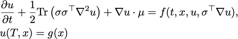
Since this article does not aim to delve into in-depth mathematical discussions, we will omit a detailed explanation of these symbols. Instead, we highlight some important aspects of this equation:

• The PDE involves a differential operator incorporating the Hessian of the solution (∇^2 u).
• The PDE involves a certain form of nonlinearity (f).
• The PDE is subject to a terminal condition.

Such PDEs correspond with Backward Stochastic Differential Equations (BSDEs) in the form below.

For a more detailed explanation of such a correspondence between PDEs and BSDEs, see [1] for example.

Examples

The deep PDE algorithms will input parameters and variables in Backward Stochastic Differential Equations defined above and output the value of function u at the initial time step (t=0), which represents the option price at the trading time. Now, let us discover the algorithms in our comparison experiments briefly. 

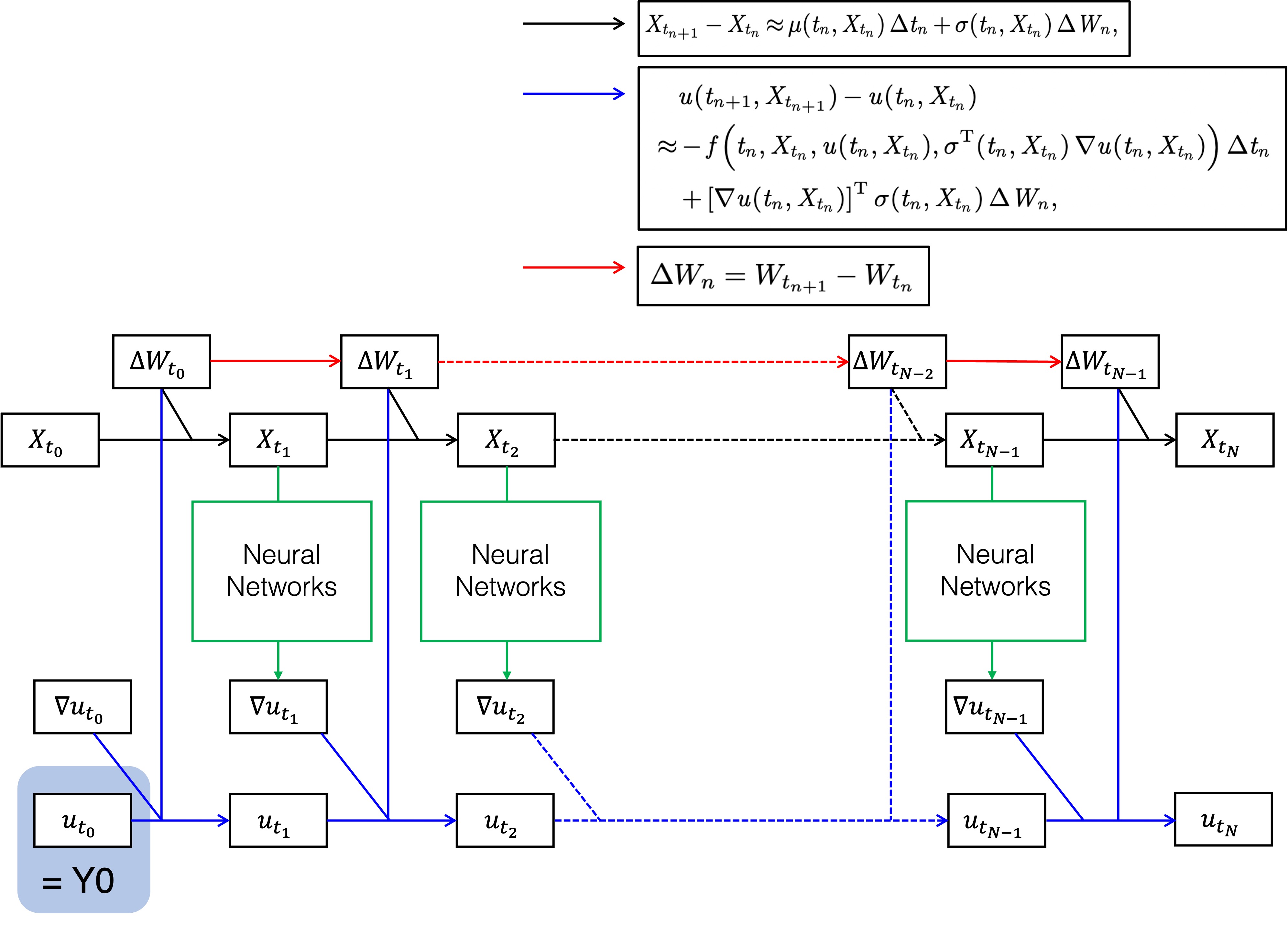
Deep Backward Stochastic Differential Equation (DBSDE) [1]

This algorithm is operated as in the architecture below. Discretizing the BSDE formula, the goal to find u at the zeroth time step transforms into the problem to find ∇u at each time step. DeepBSDE leaves that task to feedforward neural network, indicated by green blocks below. After optimizing all neural networks simultaneously to minimize the stated loss function, the initial value of u is computed. In option pricing, this value is the estimated option price. 

Deep Backward Dynamic Programming (DBDP 1/2) [3]

In this method, the training process is different, although the architecture and the discretized formula is the same. In this approach, the neural network is responsible for predicting both u and σᵀ∇u at each time step or predicting u at each time step before deriving ∇u using automatic differentiation (DBDP1 and DBDP2, respectively). More details are given in Subsection 3.2 of [3]. 

More than that, we also tested an acceleration scheme-enhanced version of DBSDE [2], Deep Splitting (DS) [4], and Multi-Deep Backward Dynamic Programming (MDBDP) [5]. 

Experiments and Results

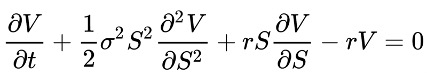
Firstly, for the low-dimensional case, we performed an experiment on the Black-Scholes Model, which means we solved the Black-Scholes Equation with specific parameters for non-dividend-paying stock, and we applied the same configuration as [1]. The PDE is given below. Here, we discretize the time into 40 steps, and we apply the learning rate of 0.08. 

The option we want to price is a European call option, which is an option that allows buying an asset at the strike price only on the date of expiration. The payoff of the option is the value of option V as the spot price is S at the expiration time T. An option will have a value only when the spot price S is higher than the strike price K; it will not be worth using the option otherwise. Therefore, the terminal condition is defined as follows.

Then, our question is formulated to find the value of V, given the initial spot price S and initial time T=0. In other words, V(S,0) represents the option price that one buys  (on Day 0). 

These are the definitions and assigned values for this experiment:

• V(S,t): price of the option 
• S(t): stock price (or any other asset’s price)
• r: risk-free interest rate = 1% per year
• σ: volatility of the stock = 0.3
• K: strike price = 90
• S(0) = 100
• T: time to expiration = 1 month

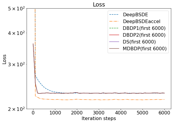
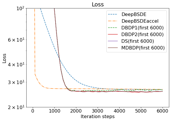
By running the experiment, we can observe the iteration of all algorithms as the loss function decreases; a graph is given below. Note that the hyperparameters cannot be kept the same across forward schemes and backward schemes because of the difference in nature between them. However, we keep them the same as possible within the same scheme. 

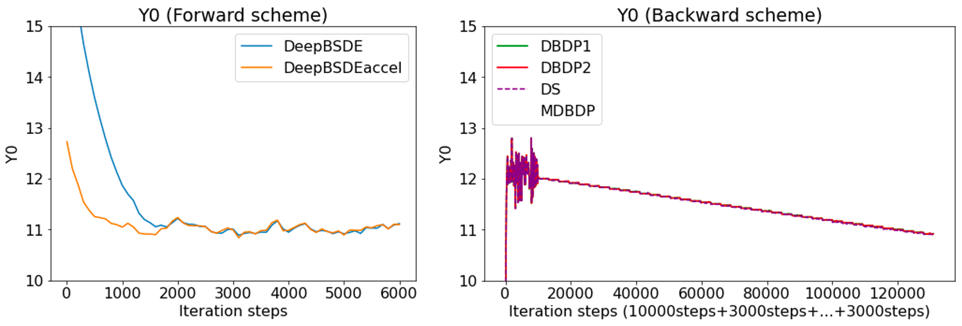
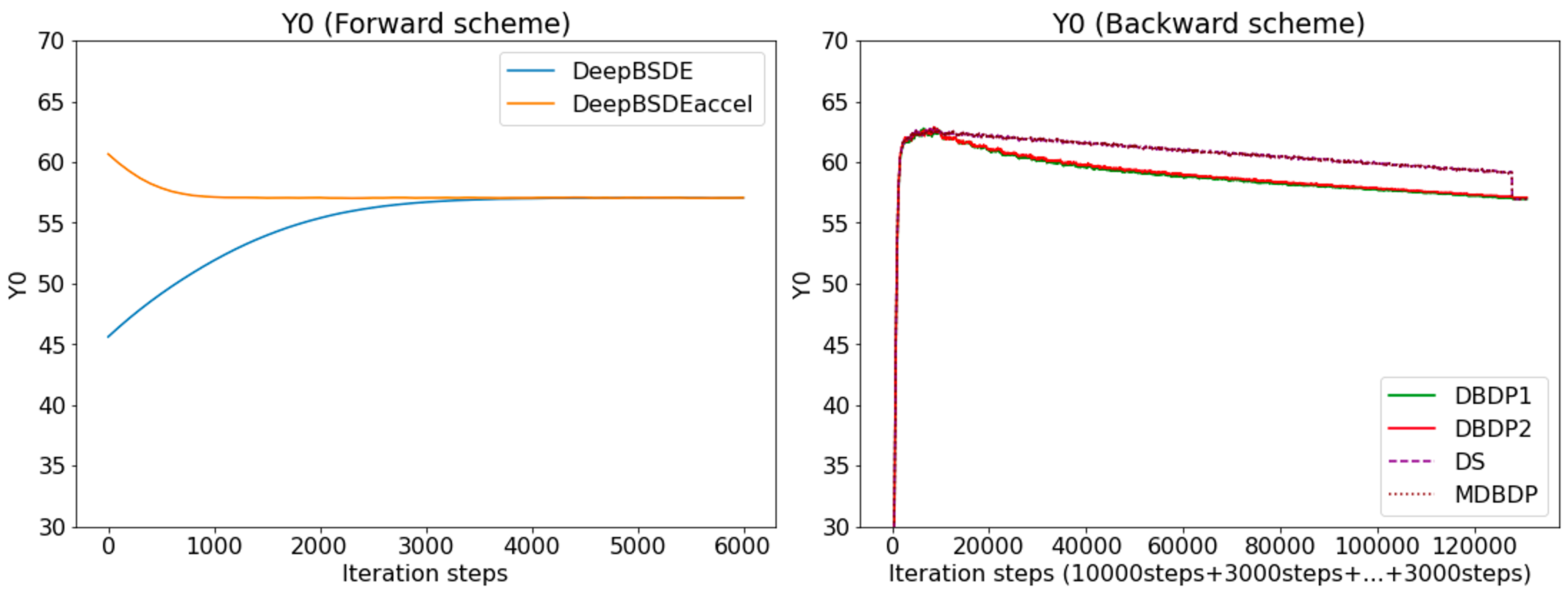
The learning of the solution (denoted as Y0; we are finding the price of the option at t=0) toward target values is illustrated below. The known explicit solution is around 10.52. In the left figure, the results from forward scheme algorithms are illustrated. In the right figure, the results from backward scheme algorithms are illustrated, but we omit MDBDP data to show results from other algorithms clearly. In the backward-scheme figure, the x-axis denotes the merged iteration steps from the initially trained time step (10000 iterations) and subsequent time steps (3000 iterations each). In both graphs, solution Y0 approaches the known solution as time goes on. After the first 10000 iterations, each of the algorithms shows the value of u at time steps 39, 38, 37, and so on, which are decreasing. Later, at the last 3000 iterations, the value at the first time step, which corresponds to the option price, is computed.

Here, the summary of each algorithm’s performance is reported below. In the table, the second column illustrates the yielded results, which are used for calculating the error in comparison with the known solution of around 10.52. In the last column, the time required to obtain the solutions is reported. 

	u(t=0)	Error (from the known solution)	Time used (s)
DeepBSDE[1]	1.1118E+01	5.69%	588.967
DBSDE + Acceleration [2]	1.1098E+01	5.50%	588.788
DBDP1 [3]	1.0925E+01	3.86%	805.575
DBDP2 [3]	1.0919E+01	3.80%	599.069
DS [4]	1.0910E+01	3.71%	596.184
MDBDP [5]	1.1249E+01	6.93%	3531.508

Here, we could find out that the backward schemes except MDBDP give a more accurate number, while they generally require longer computational time. Comparing backward-scheme algorithms, we found out that MDBDP requires a much longer time while not contributing to improving the error in this case. On the other hand, DBDP2 and DS offer the same level of error while using the same computational time. 

 

Another test is for a high-dimensional case, where we use the Black-Scholes Equation with Default Risk, with a dimension of 100 and time steps 40. We applied the same configuration and equation as the Nonlinear Black-Scholes Equation with Default Risk example in [1]. In this case, the equation has the default risk (risk of bankruptcy) term. There are plenty of ways to model it in the equation.  

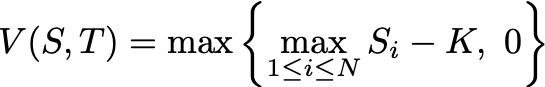
We use the best-of option, which means the payoff is defined as follows, where S_i is the spot price of each asset i. Therefore, the terminal condition for the PDE above is given below. 

In this case, there is no known analytical solution, which means we cannot compute the error by contrasting it with the known solution. Thus, we shall compute the algorithm by running the experiment 10 times and calculating the standard deviation to find its consistency. 

The convergence toward target values is illustrated below. Here, the explicit solution is unknown, but we can compare how fast each method converges by taking its final value.

Here, the summary of each algorithm’s performance is reported below. In this experiment, since there is no known, correct solution, we evaluate each algorithm by running multiple times and finding how much each run deviates from its mean. Therefore, ten runs were conducted, and both the mean and the standard deviations were reported. Additionally, we report the time used and the time required before each model converges to ±1% of the final answer. 

	Mean of u(t=0)	STD of u(t=0)	Avg. Time used (s)	Avg. Time to reach ±1% of final value (s)
DeepBSDE[1]	5.7052E+01	0.0572	675.9	316.2
DBSDE + Acceleration [2]	5.7066E+01	0.0572	763.9	82.1
DBDP1 [3]	5.6955E+01	0.147	2136.7	1764.5
DBDP2 [3]	5.7091E+01	0.151	1910.4	1582.0
DS [4]	5.6955E+01	0.687	1922.0	1875.5
MDBDP [5]	5.7180E+01	0.259	5464.3	5250

Firstly, we found that although each algorithm offers different efficiency, we cannot speak of the superiority of the forward scheme and backward scheme the fact that both require different sets of hyperparameters. Therefore, it makes sense that DBDP1, DBDP2, DS, and MDBDP take longer time to run as they train networks at each time step differently. Additionally, considering the results from the forward scheme experiments, we could confirm that the acceleration scheme [2] could help approximate the solution to initialize the neural networks; as a result, the model converges faster, as indicated by the shorter time in the last column. 

Conclusion

In summary, we could use all of the investigated algorithms to solve the Black-Scholes equation in two different scenarios – low-dimension (1-asset, Plain Vanilla call options) and high-dimension (100-asset, Call options with default risk). In both cases, all algorithms could successfully converge near the solution. Nonetheless, some algorithms were found to be more accurate than others. 

Anyway, the experimental results presented in this blog are only made with a specific set of hyperparameters. The results could change significantly if we change the neural networks model, learning rate, time discretization, epochs, etc. 

In the end, I would like to thank you for reading this blog until this point. I would like to thank all the people at PFN who have supported me during this wonderful time, especially my mentors, Minami-san and Imos-san, for your supervision. 

References

[1] Jiequn Han, Arnulf Jentzen, and Weinan E (2018). Solving high-dimensional partial differential equations using deep learning. In Proceedings of the National Academy of Sciences, 115(34), 8505-8510. https://doi.org/10.1073/pnas.171894211

[2] Riu Naito and Toshihiro Yamada (2020). An acceleration scheme for deep learning-based BSDE solver using weak expansions. International Journal of Financial Engineering, 7(2), 2050012. https://doi.org/10.1142/S2424786320500127

[3] Côme Huré, Huyên Pham, and Xavier Warin (2020). Deep backward schemes for high-dimensional nonlinear PDEs. Mathematics of Computation, 89, 1547-1579. https://doi.org/10.1090/mcom/3514

[4] Christian Beck, Sebastian Becker, Patrick Cheridito, Arnulf Jentzen, and Ariel Neufeld (2021). Deep splitting method for parabolic PDEs. SIAM Journal on Scientific Computing, 43(5), A3135-A3154. https://doi.org/10.1137/19M1297919

[5] Maximilien Germain, Huyen Pham, and Xavier Warin (2022). Approximation Error Analysis of Some Deep Backward Schemes for Nonlinear PDEs. SIAM Journal on Scientific Computing, 44(1), A28-A56. https://doi.org/10.1137/20M1355355