Blog

Home
Blog
Change Detection and its Variable Selection in Multivariate Time Series Using aHSIC with Improvements on the Algorithm

2021.11.24

Change Detection and its Variable Selection in Multivariate Time Series Using aHSIC with Improvements on the Algorithm

Area

Machine Learning / Deep Learning

Tag

# Anomaly Detection

# Internship

Motoki Sato

Engineer

This article is contributed by Ryo Yuki, who worked for the 2021 PFN Summer Internship.

Abstract

I am Ryo Yuki, a Ph.D. candidate at the Department of Mathematical Informatics at the University of Tokyo. I participated in the summer internship program in 2021 at Preferred Networks Inc. In this internship, I worked on change detection and its variable selection with my mentors.
In the robotics, medicine, economy, and various situations, there are serious risks such as malfunction, disease, and economic crisis. There has long been a need to detect and prevent these risks. These risks are often accompanied by “changes” in sensor values, diagnostic data, stock prices, etc. The issue of change detection has been studied for a long time (Basseville and Nikiforov, 1993). Recently, the variable selection of change detection has been studied. This theme assumes that time-series data is multi-dimensional and aims to not only detect changes but also to identify the anomalous variables.
One of the major problems of change detection in multi-dimensional time series is that multi-dimensional time series can be “sparse,” (Barddal et al., 2017) i.e., the variables where changes are occurring are assumed to be small compared to the number of dimensions (Figure 1). For example, in the previous example of robotics, only some robot parts likely fail rather than the entire robot. However, it is not easy to identify the changing variables, where only a few are mixed in with the variables with no changes.

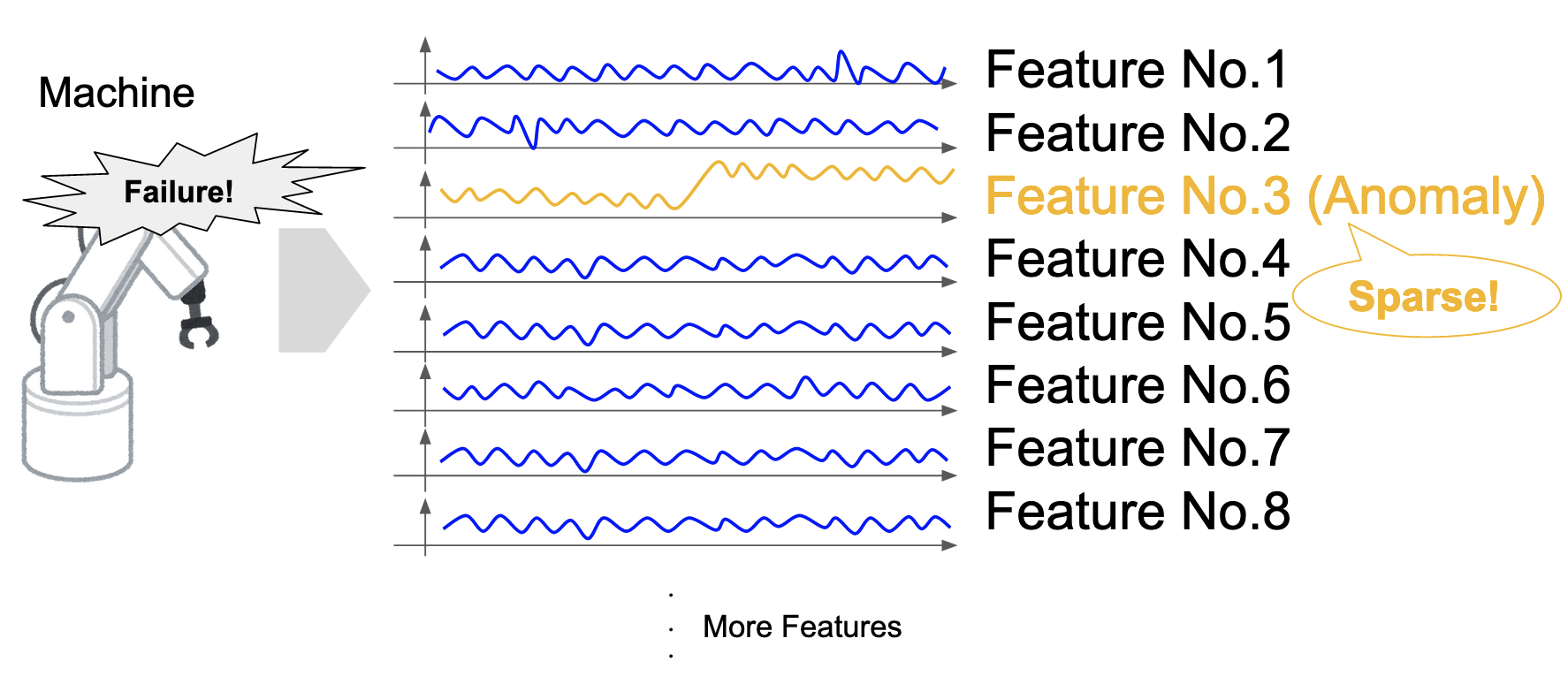
Figure 1: Sparsity of change in a multi-dimensional time series.

In this project, we investigated and implemented a change detection method called additive Hilbert-Schmidt independence criterion (aHSIC, Yamada et al., 2013), based on the kernel method and Lasso (Tibshirani, 1996; Tibshirani, 2011). To improve the performance of the method, we made the following improvements: (1) searching for multiple points in a window, (2) extension of aHSIC to handle gradual changes, and (3) automatic adjustment of the regularization factor \(\lambda\). Finally, the improved performance of the method was confirmed by experiments.

Methods

Definition of changes

In aHSIC, a change is defined as follows: Let \(X\) be the d-dimensional random variable of the time-series data. It is assumed that time \(t\) is the only candidate point of changes. A new variable \(y\) is defined as a random variable that is +1 before time \(t\) and -1 after \(t\). The time \(t\) is defined as a change point if and only if \(X\) and \(y\) are dependent (Figure 2). By artificially defining a new random variable \(y\), Lasso can be used as described later.

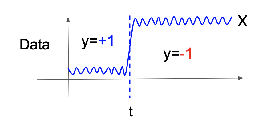
Figure 2: \(X\), \(y\), and the candidate of changes.

aHSIC

\[
\mathrm{aHSIC}(X,y)=\sum_{k=1}^d \alpha_k \mathrm{HSIC}(X_k,y),
\]

where HSIC is a non-negative measure that quantifies the dependence of two random variables (Gretton et al., 2005), \(X_k\) is the kth dimension of \(X\) over all time points, and \(\alpha=(\alpha_1, …, \alpha_d)\) are the non-negative weights and sum to 1. There are several possible ways to set the weights (e.g., set them all as \(1/d\)), but they are set by solving the following optimization problem (HSIC Lasso, Yamada, et al., 2014):

\[
\min_{\alpha \in R^d} || \bar{L}-\sum_{k=1}^d \alpha_k \bar{K}^{(k)} ||_{Frob}^2 + \lambda ||\alpha||_1, \mathrm{s.t.} \ \alpha_1, \dots , \alpha_d \geq 0, \ (1)
\]
where \(\bar{L}\) is the centered and normalized Gram matrix of \(\bar{K}^{(k)}\) is that of \(X_k\) (see the original paper for detailed definition), and \(\lambda\) is the coefficient that determines the strength of the regularization. The first term can be expanded as follows, which makes its meaning clearer:

\[
|| \bar{L}-\sum_{k=1}^d \alpha_k \bar{K}^{(k)} ||_{Frob}^2 =\underline{\mathrm{HSIC}(y,y)}_{(1)} – \underline{2 \sum_{k=1}^d \alpha_k \mathrm{HSIC}(X_k,y)}_{(2)} + \underline{\sum_{k,l=1}^d \alpha_k \alpha_l \mathrm{HSIC}(X_k, X_l)}_{(3)}.
\]

For the first term, HSIC is a constant with respect to \(\alpha\); thus, we can ignore it. For the second term, since HSIC is non-negative, minimizing the original optimization problem makes \(\alpha_k\) small when \(X_k\) and \(y\) are independent (i.e., when \(X_k\) has no change). This means that dimensions that are irrelevant to the change are removed. For the third term, minimizing the original optimization problem makes \(\alpha_k\) or \(\alpha_l\) smaller when \(X_k\) and \(X_l\) are dependent. This means that redundant dimensions are removed for the change. In summary, only the dimensions that are intrinsic to the change will remain. Finally, \(\alpha\) is normalized so that the sum is equal to 1.

Group Lasso

There is a type of multi-dimensional time series in which variables can be grouped. For example, let’s consider a machine consisting of several parts. We can group the dimensions of the time series obtained from the sensors into different parts. Rather than applying regularization to each dimension, it is natural to apply regularization to each group and set \(\alpha\) to 0 for each group (Figure 3). To this end, aHSIC based on Group Lasso (Zou and Hastie, 2005; Meier, Geer, and Bühlmann, 2008) has also been proposed. This can be easily achieved by simply changing the regularization term in Equation (1) (Reference of Group Lasso in Japanese: https://tech.preferred.jp/ja/blog/group-lasso/ ).

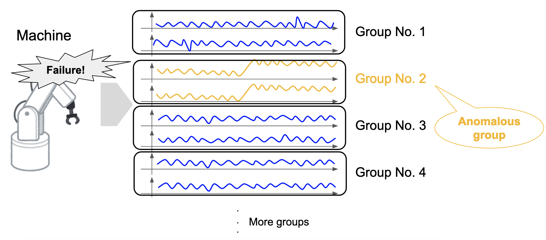
Figure 3: Concept of Group Lasso.

Sliding windowing algorithm

In real applications, it is sometimes necessary to detect the change point in an online manner. To this end, the sliding windowing algorithm is adopted (Figure 4). A certain size of data, a window, is cut from the time series data. The change score is calculated assuming the center of the window is the candidate change point. Finally, the change score is repeatedly calculated by shifting the window one by one.

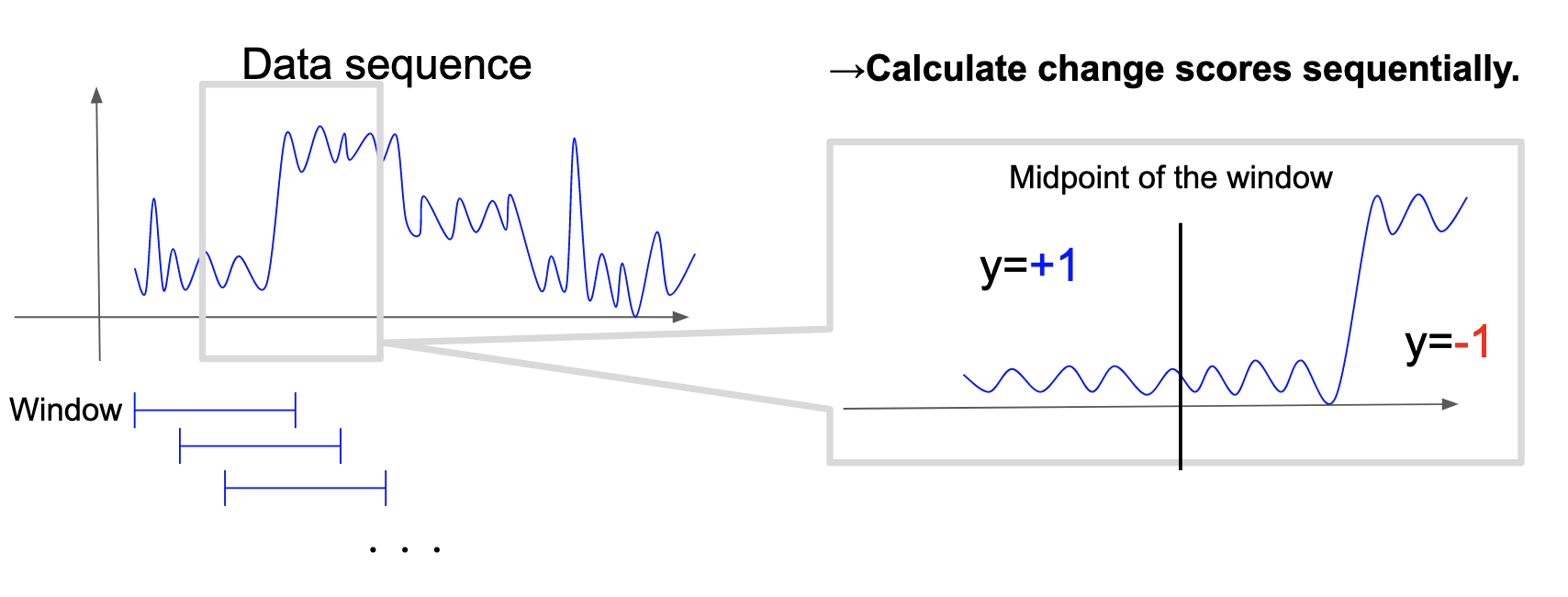
Figure 4: Concept of sliding windowing algorithm.

Improvements of aHSIC

Our proposed improvements of aHSIC can be summarized as follows: (1) searching for multiple points in a window, (2) extension of aHSIC to handle gradual changes, and (3) automatic adjustment of the regularization factor \(\lambda\).

1. Search for multiple points in the window

In the original algorithm, the change score is calculated assuming that only the midpoint of the window is the change point. However, there is always a gap between the true change point and the midpoint because the latest data is always coming in from the right side, which reduces the reliability of the change scores. Therefore, the algorithm was changed to assume that various points in the window are candidates for changes and output the maximum change score and its corresponding contribution rates.
Furthermore, suppose all points in the window are assumed to be change candidates. In that case, the computational complexity is multiplied by the size of the window, which makes the algorithms time-consuming. Therefore, t-1, t-2, t-4, t-8, etc., are assumed to be change candidates, where \(t\) is the latest time point. In this way, the score for the change points coming in from the right is accurately calculated while keeping the multiplication in computational complexity to the logarithm order of the window size (Figure 5).

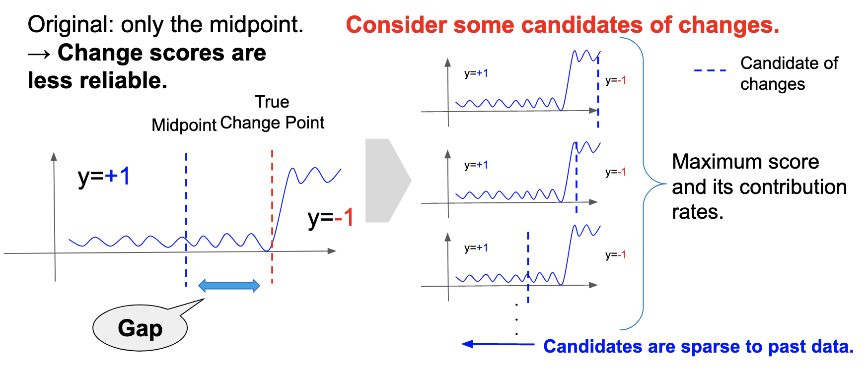
Figure 5: Concept of the improvement on the algorithm.

2. Extension of aHSIC to handle gradual changes

Conventional change detection methods assume that abrupt changes occur, i.e., the parameters inside the probability distribution followed by the time series data change all at once after a certain time (Basseville and Nikiforov, 1993; Gralnik and Srivastava, 1999; Takeuchi and Yamanishi, 2006; Adams and MacKay, 2007; Saatçi, Turner, and Rasmussen, 2010). This is because they are statistically tractable. However, in the real world, a gradual change, that is, a type of change in which the parameters of the probability distribution change gradually over a certain range of time, is also considered to occur (Figure 6). Since the parameters change gradually, it is more difficult to detect such changes than the conventional abrupt changes. Several studies that detect the starting points of gradual changes have been conducted (Yamanishi and Miyaguchi, 2016; Yamanishi et al., 2020).

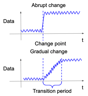
Figure 6: Example of abrupt and gradual changes.

The occurrence of abrupt changes is implicitly assumed in aHSIC. Thus, we changed \(y\) to correspond to gradual change, as shown in Figure 7. Specifically, the candidate of the abrupt change in the original method was considered to be the candidate of the starting point of the gradual change, and \(y\) was reformulated to increase linearly from the starting point.

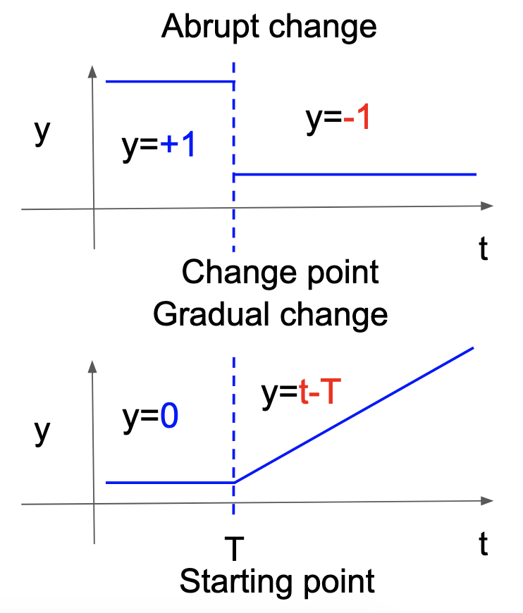
Figure 7: Formulation of \(y\) in abrupt and gradual changes.

3. Automatic adjustment of regularization factor \(\lambda\)

The proposed method has several hyperparameters. Among them, the hyperparameter \(\lambda\), which determines the strength of the regularization, has a particularly large influence on the performance of the proposed method. How can we tune \(\lambda\)? One way is to determine a quantitative evaluation index for change detection and variable selection performance and divide the given time series data and change labels into validation and test datasets. However, in many cases, it cannot be guaranteed that no changes have occurred even at points that are not labeled as change points (e.g., overlooked changes during label creation), which makes the negative labels for time series data less reliable. Therefore, the change detection methods should have a low dependency on the hyperparameter change labels. To solve this problem, we propose to use grid search and k-fold cross-validation (CV) to determine \(\lambda\) for the first term of the loss function in Equation (1). We can determine \(\lambda\) while using time series data and reducing the dependence on change labels.

Experimental Results

Three experiments were conducted to evaluate the performance of the above three improvements.

Evaluation metrics

It is assumed that a time series of data, the true change points, and the variables with changes are given. The aHSIC method outputs uni-dimensional change scores and multi-dimensional contribution rates. Change detection is evaluated by the area under the curve (AUC) with the change scores. Variable selection is evaluated by mean average precision (MAP) with the contribution rates.

AUC

AUC is an effective measure for binary classification if the ratio of positive and negative cases is imbalanced. Usually, in change detection, it is assumed that the portion of changes is much less than that of data without changes. Thus, AUC is considered effective for evaluation. The data at and near the true change point are treated as positive examples, whereas the other data are treated as negative examples (Figure 8).

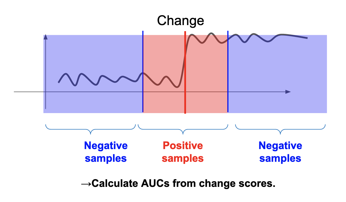
Figure 8: Settings of positive and negative samples for the calculation of AUC.

MAP

The variable selection was evaluated using MAP. The higher the contribution rate of aHSIC, the more likely it is that a change is occurring. Thus, we can use MAP, which is a metric used in, for example, ranking learning and object detection (Figure 9). Our experiments extracted the contribution rates of only the true positive samples to calculate MAP.

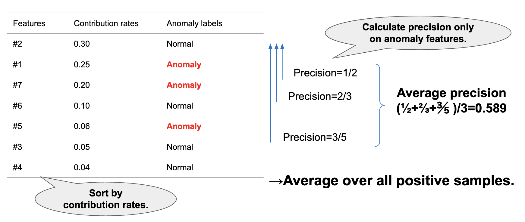
Figure 9: Calculation of MAP.

Artificial Datasets

Two types of data, ungrouped and grouped data, were used. First, 50-dimensional data sequences, which had 2000 data points, were generated. Each data point independently followed a normal distribution N(0,1). Then, we grouped the data by five dimensions and divided them into ten groups. Next, we selected five dimensions from the 50 dimensions as the dimensions with changes for both types of the data sequences. For the ungrouped data, five groups were randomly selected, and one dimension was selected from each group as the dimension with a change. For the grouped data, one group was randomly selected, and all the dimensions of the selected group were chosen as the dimensions with a change. Then, for each change, we increased the mean by 3. Finally, the data were divided into equal intervals to generate 9 change points. An example of the data is shown in Figure 10.

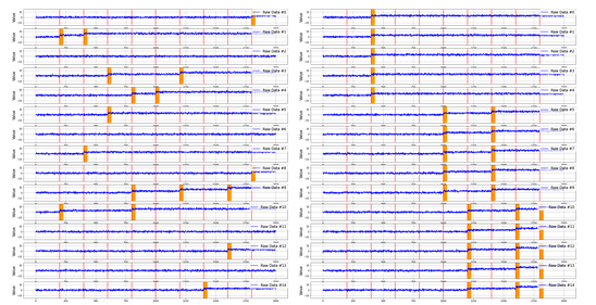
Figure 10: An example of ungrouped and grouped data. The red lines denote change points, and the orange bars denote the variables where changes occur. All the changes are abrupt changes. Left: Ungrouped data. Right: Grouped data.

To evaluate the extension of aHSIC to gradual changes in the second experiment described later, we prepared two types of data, one with an abrupt increase and the other with a gradual increase when increasing the mean by 3. In the gradual change, we set the length of the transition period to 30, and the mean increased linearly. An example is shown in Figure 11.

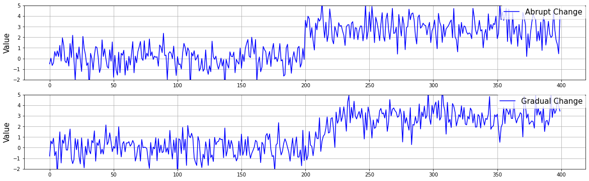
Figure 11: Abrupt and gradual changes.Top: Abrupt change. Bottom: Gradual change.

We generated 10 data sequences for each type. The parameters of the generated data are shown in Table 1. Besides, 30 data points from each change point of abrupt change and each starting point of gradual change were set as positive examples for AUC/MAP calculation.

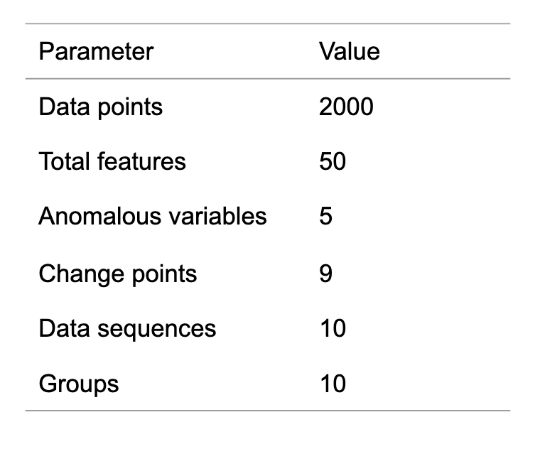
Parameters of data sequences.

Other settings

Details of the method

We have evaluated the performance of two methods: aHSIC based on Lasso and aHSIC based on Group Lasso. The coordinate descent method was used for Lasso, and the proximal gradient method was used for Group Lasso to calculate the optimal solution.
In all experiments, the kernels for calculating the centered and normalized Gram matrix of the time series data \(X\) were the radial basis function (RBF) kernels. To calculate the Gram matrix of \(y\), a delta kernel (i.e., a kernel that takes 1 when the two input variables are the same and 0 otherwise) was used for abrupt changes and an RBF kernel for gradual changes.
The hyperparameters of the method are based on the window width, kernel bandwidth (\(X\) and \(y\), respectively), and regularization factor \(\lambda\). However, for abrupt changes, no bandwidth is needed to calculate the centered and normalized Gram matrices of \(y\) because the delta kernel does not have its bandwidth.
One data sequence was used for adjusting the hyperparameters (i.e., validation data) and the remaining nine data sequences for the test dataset. How to tune the hyperparameters is given in the next section.

Hyperparameter tuning

When considering the real-world applications of variable selection, both the change and the variable identification should be done well simultaneously, and it is not very meaningful if only one of them is done well. Therefore, we performed a bivariate optimization of AUC and MAP using the tree-structured Parzen estimator sampler (TPE, Bergstra et al., 2011) implemented in Optuna (Akiba et al., 2019). Subsequently, the hyperparameters were set to optimize AUC+MAP (Figure 12).

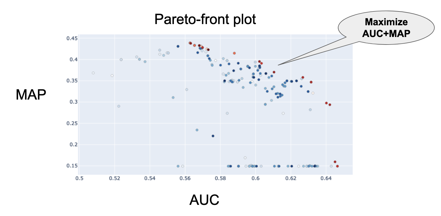
Figure 12: Pareto-front plot of AUCs and MAPs.

Under the above settings, the following three experiments were conducted. In each experiment, we evaluated how much each of the three improvements improved the algorithm’s performance compared to the original algorithm, without combining any two improvements (i.e., first and second improvements).

Experiment No. 1: Improvement by searching multiple points in a window

Lasso and Group Lasso were applied to ungrouped and grouped data. The results are shown in Table 2. The result showed that the algorithm improved AUC and MAP in most cases. Although the improvement of AUC where Lasso is applied to the grouped data was not confirmed, we confirmed the improvement by referring to the sum of AUC and MAP.

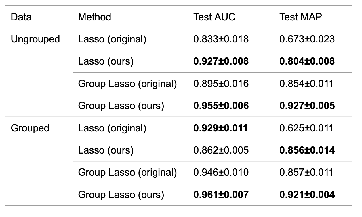
Table 2: Mean and standard deviation of AUC and MAP for the original algorithm and the proposed algorithm.

Experiment No. 2: Improvement by extending aHSIC for gradual change

For the ungrouped and grouped data, we generated two types of data corresponding to abrupt and gradual changes. In other words, a total of four types of data were generated. Next, Lasso and Group Lasso were applied. The results of applying the method to abrupt and gradual changes are shown in Table 3. The results for gradual change showed that the proposed method generally outperformed the results in the original algorithm. Interestingly, the proposed method also outperformed the original method in the case of abrupt changes.

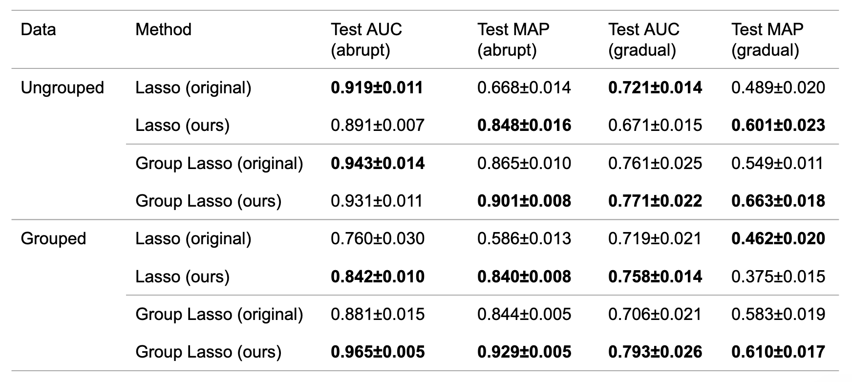
Table 3: Mean and standard deviation of AUC and MAP for the original algorithm and the proposed algorithm.

Experiment No. 3: Improvement of the regularization factor \(\lambda\) by adjusting it using CV

Lasso and Group Lasso on the ungrouped and grouped data were applied. When \(\lambda\) was adjusted using CV, the bandwidth and the window width were adjusted using Optuna. On the other hand, when \(\lambda\) was not adjusted using CV, the bandwidth, the window width, and \(\lambda\) were adjusted using Optuna. The results are shown in Table 4. In both cases, the performance of the one using CV to adjust \(\lambda\) was comparable to that of the one not using CV. Therefore, the results showed that the dependence of the method on the hyperparameters was reduced while maintaining the performance.

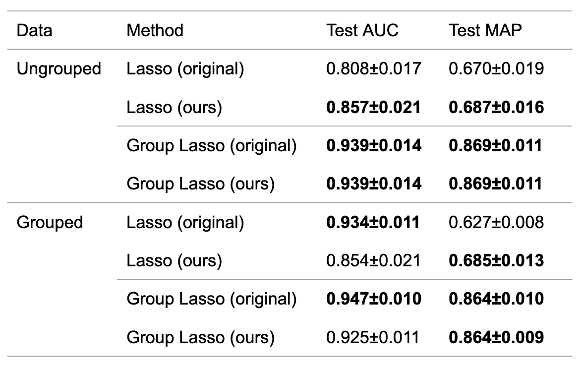
Table 4: Mean and standard deviation of AUC and MAP for the original algorithm and the proposed algorithm.

Conclusions and Future Work

We have investigated change detection and variable selection. We made three improvements to the aHSIC method: (1) searching for multiple points in a window, (2) the extension of aHSIC for gradual changes, and (3) the automatic adjustment of the regularization factor \(\lambda\). In the first two points, AUCs and MAPs were improved. In the last one, we confirmed that the method’s dependence on the anomaly labels was reduced while maintaining the performance.

The following problems remain for future study:
Performance analysis of the anomalous variable selection. In change detection, there are two indicators to evaluate the performance: false positives and false negatives. False positives are defined as raised alarms even though there is no change, and false negatives are defined as overlooked changes. Several studies have analyzed the theoretical performance of these measures. However, in the present problem setting, we further identify the variables where the changes occur. Therefore, the theoretical performance analysis on variable selection and its consistency with sufficiently large numbers of data points should be analyzed.

Automatic adjustment of hyperparameters. In this article, we have introduced a method to automatically adjust \(\lambda\) by minimizing the first term of Equation (1). Although promising results have been obtained experimentally, it is still unclear that minimizing the first term of Equation (1) means optimizing AUC and MAP. The relationship between the two needs to be clearer. Besides, aHSIC has two other parameters, the window width, and kernel bandwidth. As for the window width, an adaptive windowing method (Bifet and Gavalda, 2007) has been proposed, and we can combine it with this method. As for the bandwidth, since it commonly appears in kernel methods, some general adjustment methods can be used.

Clarification of the phenomena identified in Table 3. In the second improvement, we extended aHSIC to the detection of gradual changes. It is interesting to note that while the detection performance for gradual changes has improved, the performance for abrupt changes has also generally improved. The reason for this needs to be clarified.

Acknowledgements

I was able to have a very fulfilling internship thanks to the support of the employees at Preferred Networks Inc. My mentors, Sato-san and Mori-san, were especially helpful in discussions about methods and implementation. Komatsu-san and Kume-san in the same team gave me many valuable comments at meetings. Thank you very much. Finally, I would like to express my deepest gratitude and appreciation to all the people with whom I was involved in this internship.