This article is contributed by Jinzhe Zhang, who worked for the 2021 PFN Summer Internship.

Introduction

The traditional drug discovery technique often involves a trial-and-error process and most of the candidates are chemical compounds that have been found in nature. For example, up to 2014, 49% of small-molecule cancer drugs were either natural products or their derivatives [1].

This trial-and-error paradigm contains two major drawbacks: 1) the molecule collections present in nature are only a tiny fraction of all theoretically possible molecules, 2) it is not realistic to exhaustively test or simulate the property of each candidate and there is no evident way to accelerate the searching. While researchers are dedicating their best to find a remedy for untreated diseases. Patients are still suffering while waiting. There is both an economic and a social need to improve and accelerate the current drug discovery process.

Applying Machine Learning or AI based methods to help the drug discovery process has been a hot topic for the recent years [2]. In a previous tech blog, PFN has announced the discovery of several non-peptidic compounds that can successfully inhibit SARS-CoV-2 Mpro protein using AI-driven drug discovery. Most of the AI based drug design models involve a combination of generative models and optimization methods. One major branch among branches of AI based generative models is Variational Autoencoder (VAE) [3]. In this blog, I will first introduce how VAE can be applied in the context of drug design and how the “weighted retraining” technique [4] can improve the results of VAE based models. Then, I will introduce my results of the experiments on the “weighted retraining” technique performed during my internship in PFN, and discuss our understanding on the effectiveness of this method.  

Variational Autoencoder

Autoencoder is an unsupervised learning method which leverages neural networks to force information through a bottleneck in order to learn meaningful representation. An autoencoder (AE) model typically contains two networks: an encoding network and a decoding network. The encoder is trained to map the high-dimensional input data into a vector in a lower-dimensional space, known as the latent space, and the decoder is trained to map the vector back to the exact input data. This training process can be achieved by minimizing a reconstruction loss \(L(x_i, \hat{x_i})\) which represents the difference between the original input data to the encoder and the reconstructed data from the decoder. In the context of molecule design, the input can be molecule structures represented in one of the molecule representations. The goal is to ask the encoder to compress molecules into a more distilled representation form while still being able to restore the distilled information back to a molecule.

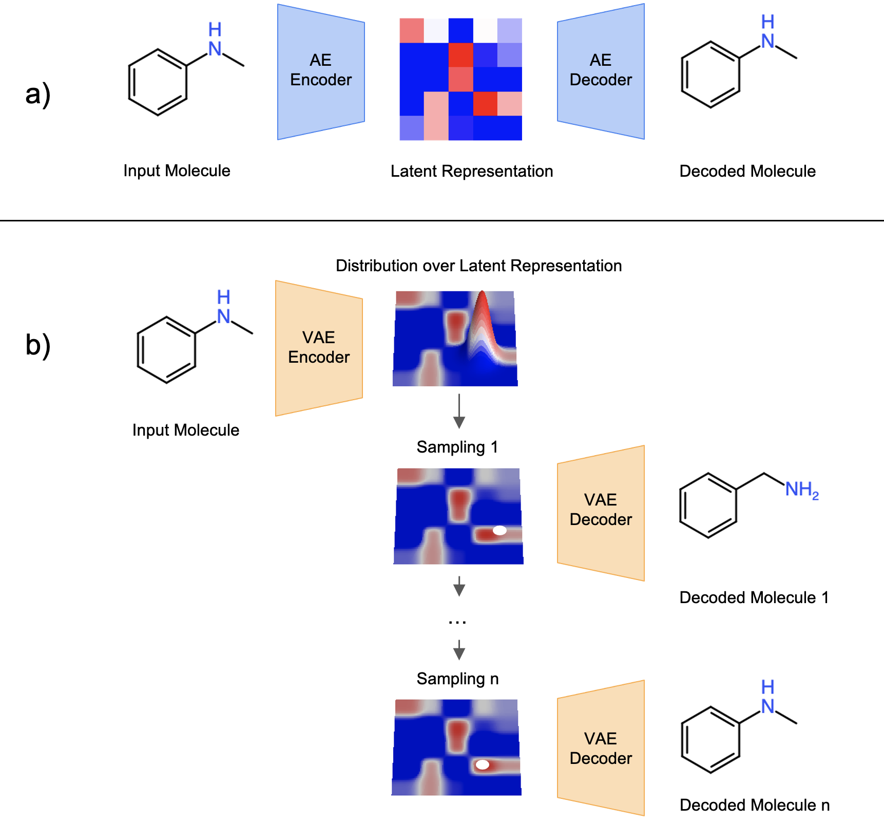
Fig. 1 Concept of a) AE and b) VAE under the context of molecule design. This figure is recreated by the author with the concept inspired from Fig. 3 of [5].

While the traditional AE is doing good on reproducing training data, it tends to learn to memorize the training data and therefore is weak on extrapolation and sampling. The Variational Autoencoder (VAE) [3] improves the generalizability issue of AE by restricting the encoder to generate latent space vectors following a probabilistic distribution. In training, a noise is added into the latent space vector to ensure the decoder can correctly reconstruct the molecule from a noisy vector. With the concept of VAE, molecule structures are expected to be “continuous” in the latent space: two latent vectors close to each other in the latent space should be translated into similar molecule structures; the farther away two latent vectors are, the more dissimilar two molecules should be. With the VAE model, the discrete chemical space can be transformed into a continuous numerical space with the benefit of having some level of molecule structure continuity and smoothness over the latent space.

To design a molecule, an inverse design process needs to be achieved: we know what property (i.e., binding affinity to a target protein)  is needed and we seek for which molecular structure(s) can give us that particular property. For VAE based molecule generation, it is often the case that a surrogate model is trained to map the latent space to the property space so that the target property can be optimized over latent space. The local and global minima will be the good drug candidates obtained by our model. This optimization process is usually called Latent Space Optimization (LSO). 

Latent Space Optimization & Weighted Retraining

 Although several optimization methods have been applied for LSO, the latent space is generally believed as hard to optimize due to several different reasons: 1) molecule structures might be smooth on the latent space, however, their property space might be rough (this phenomenon is also known as the “activity cliff” [6]); 2) good candidates may represent only a small fraction of the latent space and therefore hard to be found during optimization [4].

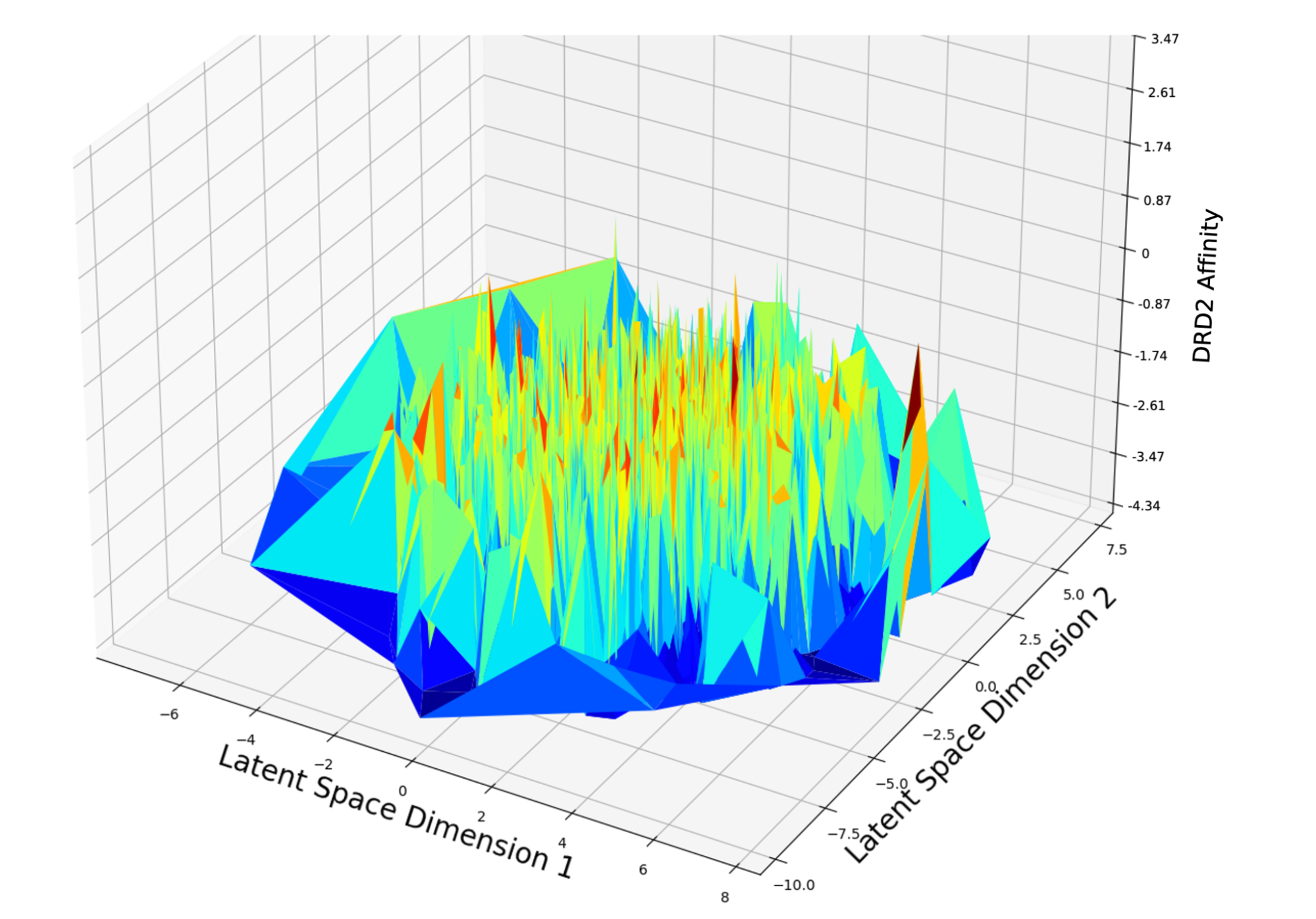
Fig. 2 Latent space is rough over property space of DRD2 Affinity

 While there is not yet a clear answer about how to construct a latent space that is optimally smooth on their property space, one study tried to tackle the second point listed above by making good candidates represent a larger fraction of volume in the latent space using a technique called weighted retraining [4].

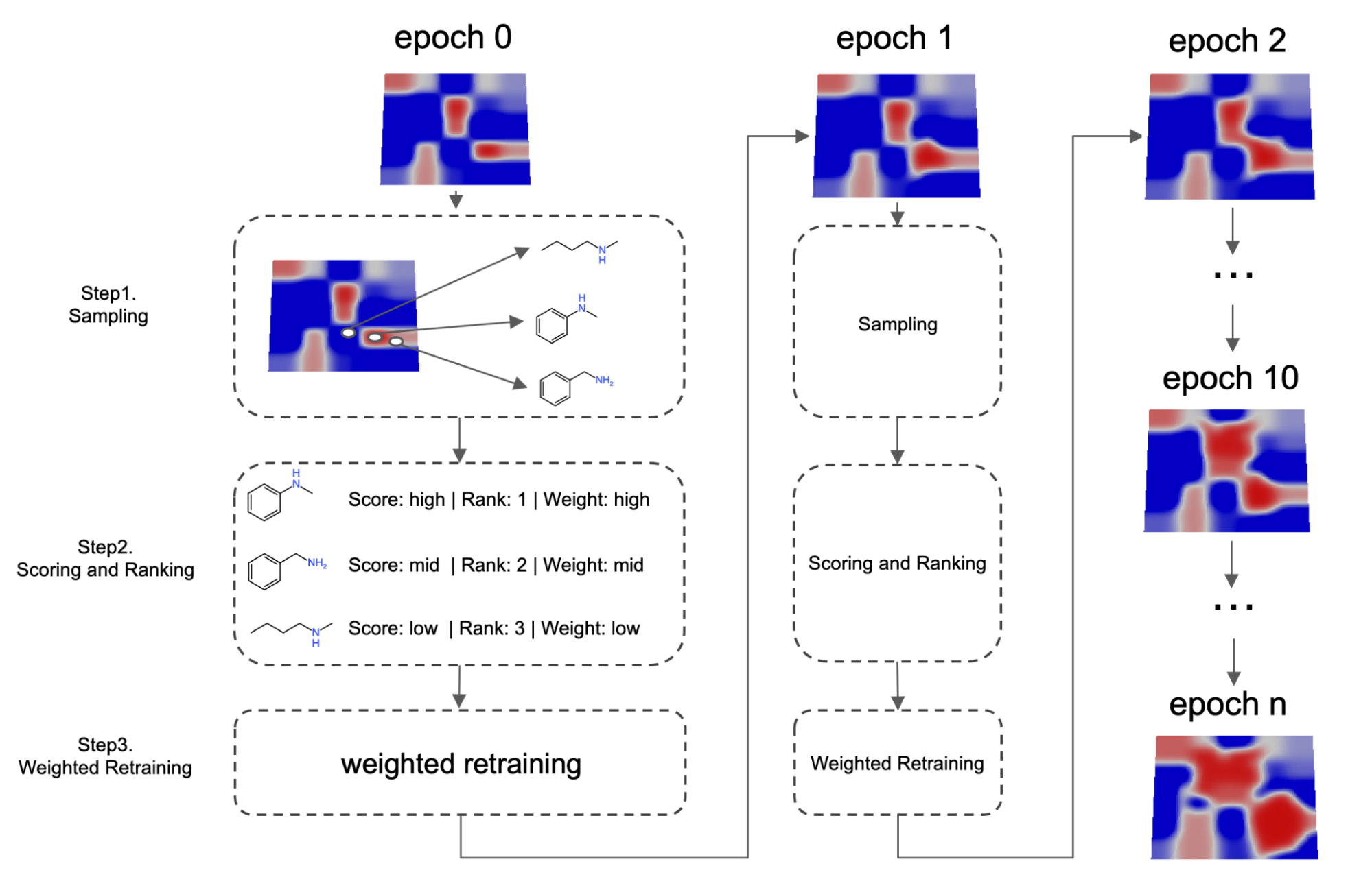
Fig. 3 Schematic illustration of the weighted retaining mechanism

Traditional Variational Autoencoder gives equal weight for every training set data. In other words, during the training, failure to reconstruct a good candidate or a bad candidate will produce equal impact on the loss. The neural network will not be in favor of one compared to the other. The concept of weighted retraining is different: a larger loss should be given when VAE failed to reconstruct a good candidate and a smaller loss when VAE failed to reconstruct a bad candidate. 

More specifically, as shown on Fig.3, the algorithm will periodically retrain the VAE. In step 1, before each retraining cycle, a set of molecules maximizing the expected property value are sampled from latent space using a surrogate model. These samples are then mixed with training set data from the previous epoch to construct a new training set. In step 2, a weight is assigned to every training set datum. This weight can be determined by a variety of methods, but in general, the weight is correlated to how good the candidate is compared to other candidates or a specific threshold. High scoring data will therefore be associated with a larger weight and low scoring data will be associated with a lower weight. In step 3, neural networks are retrained using a weighted loss: when computing the loss, the total loss is a weighted sum of each individual data. This retraining process is called weighted retraining.

Formally, the weighted loss is defined as:

\[L=\sum_{x_i \in D} w_i L(x_i, \hat{x_i})\]

with

\[W_i \propto \frac{1}{kN+\mathrm{rank}(x_i)}\]

By designing the loss function in this way, the VAE will gradually ensure that good candidates are correctly reconstructed. As the VAE needs to correctly reconstruct a noisy input following a probability distribution, good candidates will essentially take a larger volume in the latent space.

Methods

To investigate how this weighted retraining technique can impact the results of VAE based models, as a showcase experiment, I tested VAE model with weighted retraining on both penalized water-octanol partition coefficient (logP) and Dopamine receptor D2 affinity (DRD2) optimization tasks. 

Scoring Functions

In my experiments, I compare optimization performance with or without weighted retraining mechanism on two optimization tasks: one maximizing penalized logP score of the molecule, one maximizing binding affinity value against DRD2 binding. 

The penalized logP score in our experiments is calculated similarly to previous studies [7-11]. The source code can be found here. 

The DRD2 binding affinity is obtained by a GNN based predictive model. The GNN predictive model has a similar architecture to [12]. To predict the binding affinity against a specific binding, the model needs to be trained using experimental affinity data. I obtained the inhibition constant (Ki) value of different molecules from the ChEMBL database against the DRD2 binding. Smaller the Ki value represents stronger binding affinity. After deduplication and data cleaning, more than 6,000 molecule-affinity pairs remain as the training set of the GNN predictive model. The “DRD2 Affinity” in this study is defined as the following:

\[\mathrm{DRD2\ Affinity}(\mathrm{molecule})=-\log(\hat{K_i}(\mathrm{molecule}))\]

I choose to take the logarithmic value of Ki as an effort to overcome the fact that Ki values vary a lot in terms of magnitude which is suboptimal for the neural network to learn. In addition, the logarithmic value is negated so that higher “DRD2 Affinity” value represents higher binding affinity, our goal is to minimize Ki and therefore maximize this “DRD2 Affinity” value. 

VAE Model

As a popular branch of generative models, several architectures have been proposed for molecular design tasks [7, 13-15]. In this study, I choose to use JT-VAE [7], a VAE based model which encodes molecules using a junction tree based graph molecule representation, as our base VAE model similar to the original study of weighted retraining. The original implementation of JT-VAE can be found here.

Results

To demonstrate how the latent space evolves after a different number of weighted retraining epochs, let’s first compare the optimization performance on both tasks with or without weighted retraining implemented. 

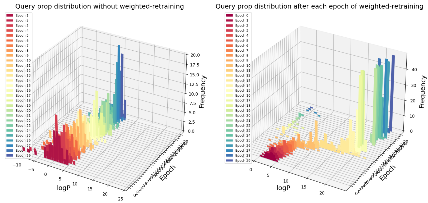
Fig. 4 Query scores distribution after each epoch of retraining with or without weighted retraining applied for logP maximization task

In Fig. 4, the first axis is the logP value of query points from optimization method, the second axis represents the number of epochs of retraining, the third axis is the histogram of query logP distribution. Our optimization goal is to maximize logP value. For each epoch, 50 points are queried from the latent space using an adaptive gradient descent method (Adagrad). On the left figure (without weighted retraining), epochs of retraining (query number) makes almost no impact on the maximum logP molecule that the model has found. In contrast, with weighted retraining, the highest logP molecule found continues to improve after a few epochs of “warm-up”. In addition, the average logP score for each epoch (50 queries) is also increasing, suggesting that not only the extreme-high logP value is improved, but also most of the queries return higher logP value molecules.

For the case of DRD2 affinity optimization (Fig.5), although less significant in terms of value, there is still an improvement of DRD2 affinity score with more epochs of weighted retraining. 

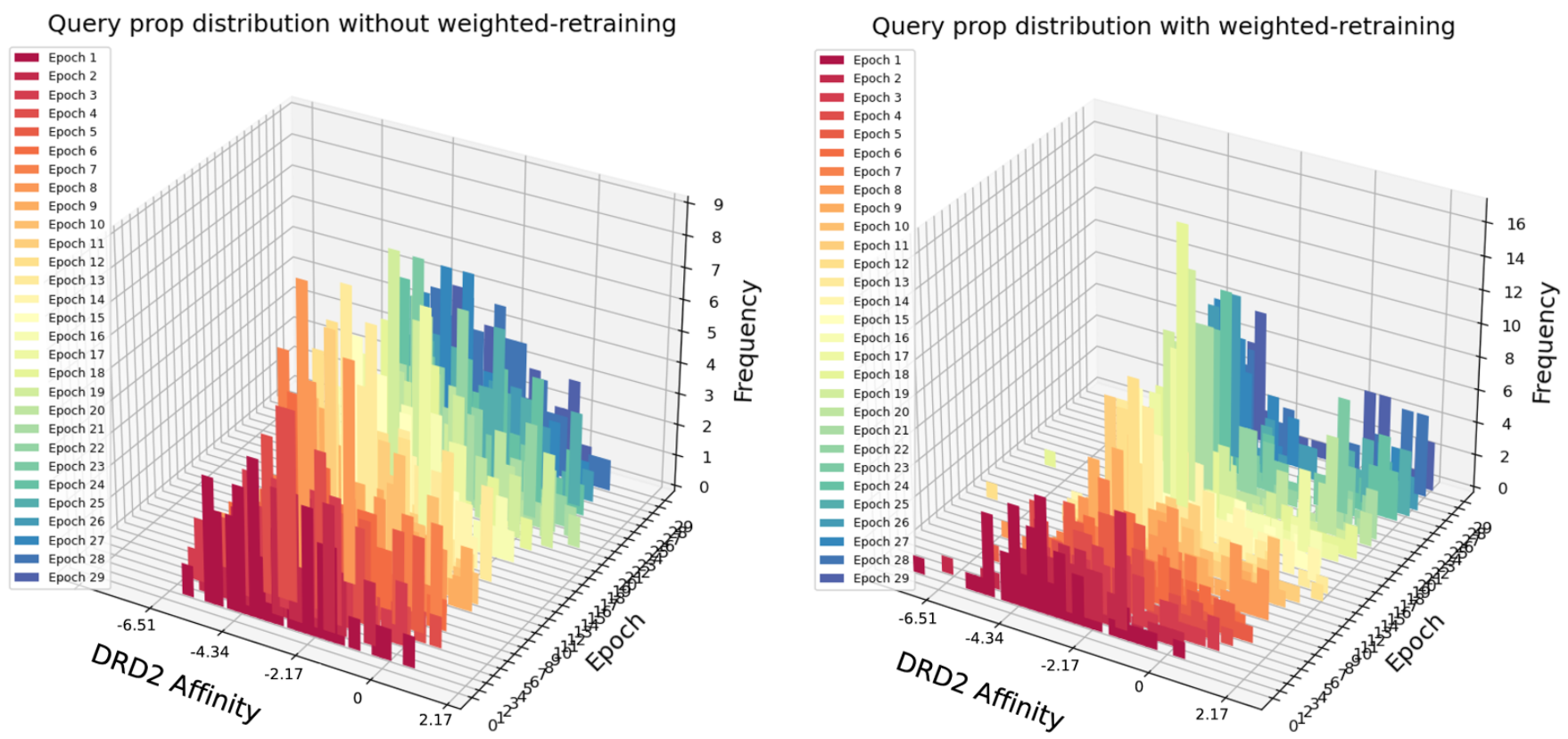
Fig. 5 Query scores distribution after each epoch of retraining with or without weighted retraining applied for DRD2 Affinity maximization task

Now we have seen how queries results over latent space have changed with weighted retraining. Let’s dig deeper and try to understand what has happened in the latent space over epochs of weighted retraining.

Below are four figures representing the logP value distribution over latent space after the 0, 10, 20 and 30 epochs of weighted retraining. In my experiments, the encoder will encode the molecular structure into a 54 dimensional latent space. In these figures, only the first and the second dimension are visualized.

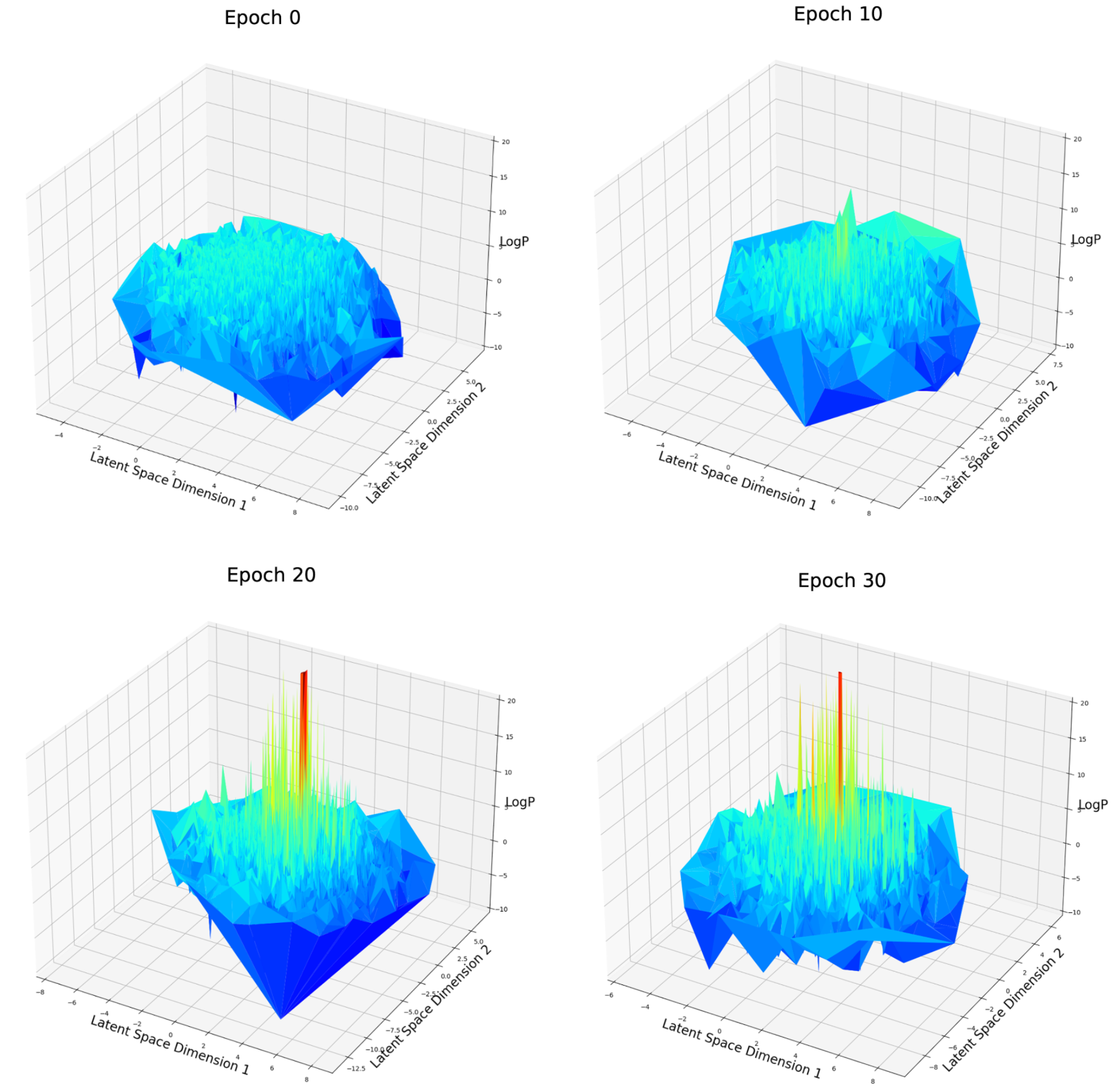
Fig. 6 LogP score distribution over first and second dimension of latent space after different epochs of weighted retraining

For the logP optimization case (Fig. 6), at epoch 0, the space is rough and contains many local maxima. There is no obvious aggregation about these local maxima. After 10, 20 or 30 epochs of weighted retraining. The logP value of several local maxima has significantly improved which corresponds to our previous observation. Depending on the mechanism of weighted retraining, high-score molecules are expected to be clustered on the latent space because weighted retraining will enlarge the volume around a good candidate. But no such aggregation is observed. One explanation about why this could have happened is that the aggregation has not happened on the first and the second dimension of latent space, but other dimensions among a total of 54. To verify this, I created a t-SNE [16] plot (Fig.7) in which all of the 54 dimensions of latent space are compressed into a two-dimensional space, all the dimensions can be overwatched at once. 

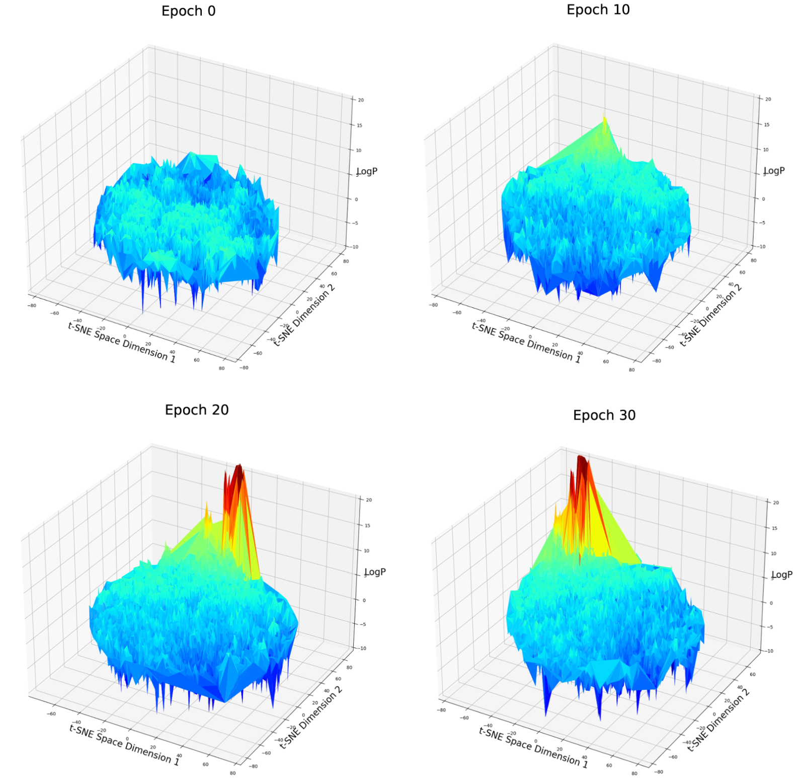
Fig. 7 LogP score distribution over 2D t-SNE compressed latent space after different epochs of weighted retraining. Note: Rotation of the t-SNE space has no meaning because each t-SNE algorithm is a random process and can not be controlled if the input data is different.

On the t-SNE plot, a clear aggregation can be observed among good candidates. This partially verified our assumption. But there is still a possibility that this aggregation is just formed because they are all extreme values of different parts of the latent space and just be aggregated by the algorithm of t-SNE. Let’s move on to the next case.

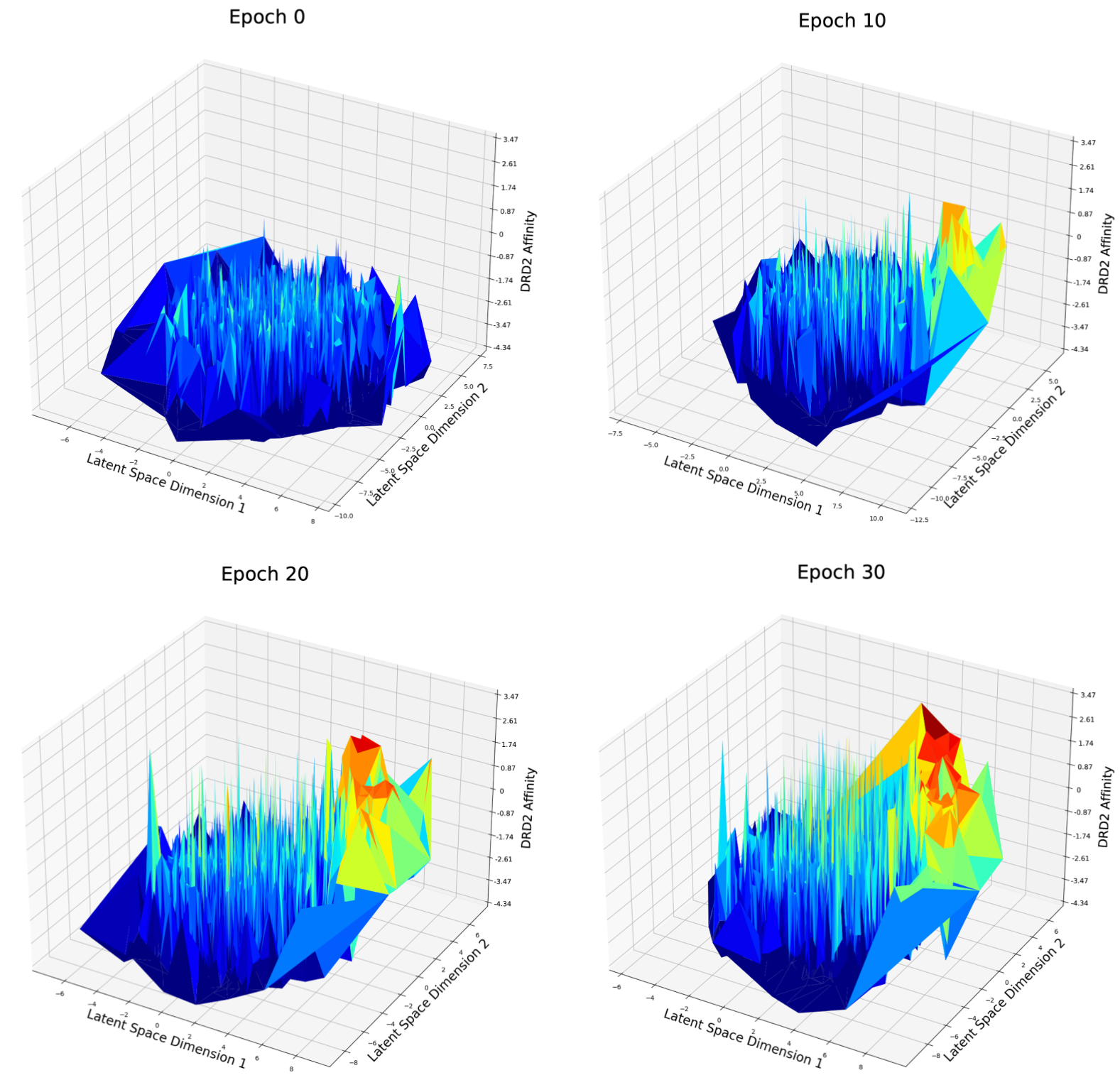
Fig. 8 DRD2 Affinity distribution over first and second dimension of latent space after different epochs of weighted retraining

For the DRD2 affinity optimization case (Fig. 8), at epoch 0, the latent space seems to be rough and good candidates are distributed randomly in the latent space. At epoch 10, a peak has grown on the right side of the figure. There are more good candidates located in the left area and the best candidates in epoch 10 have a better score compared to epoch 0. I believe this phenomenon matches what has been described in Fig. 3: with weighted retraining, the volume of good candidates will be increased, consequently, the volume of molecules around the good candidates will also be increased, so that it becomes easier for the optimization method to find a potential new good candidate nearby the current good candidate.

Conclusion

This article gave a brief introduction of VAE based molecule design, LSO and weighted retraining technique. Based on my preliminary study, it is believed that weighted retraining is an interesting technique for LSO tasks. I personally would metaform the weighted retraining technique as a magnifying glass in the latent space: it will zoom in the scope over certain areas of the latent space to make it easier to spot good candidates. However, this technique also has its drawbacks such as lack of diversity in the generated molecule structure. 

Acknowledgement

I would like to express my sincere gratitude towards people who provided critical help during my internship. Firstly, I thank my mentors: Ishitani-san and Takemoto-san for insightful mentorship, crucial knowledge and gentle encouragement. I extend my thanks to Okanohara-san, Maeda-san and Rikimaru-san for useful discussion regarding LSO and Cholesky decomposition issues. Finally, I would like to thank all the personnel from Preferred Networks Inc. that were involved in this internship. It was a wonderful journey working with you all. 

References

1. Newman, David J., and Gordon M. Cragg. “Natural products as sources of new drugs over the 30 years from 1981 to 2010.” Journal of Natural products 75.3 (2012): 311-335.
2. Sanchez-Lengeling, Benjamin, and Alán Aspuru-Guzik. “Inverse molecular design using machine learning: Generative models for matter engineering.” Science 361.6400 (2018): 360-365.
3. Kingma, Diederik P., and Max Welling. “Auto-encoding variational bayes.” arXiv preprint arXiv:1312.6114 (2013).
4. Tripp, Austin, Erik Daxberger, and José Miguel Hernández-Lobato. “Sample-efficient optimization in the latent space of deep generative models via weighted retraining.” Advances in Neural Information Processing Systems 33 (2020).
5. Bian, Yuemin, and Xiang-Qun Xie. “Generative chemistry: drug discovery with deep learning generative models.” Journal of Molecular Modeling 27.3 (2021): 1-18.
6. Dimova, Dilyana, and Jürgen Bajorath. “Advances in activity cliff research.” Molecular informatics 35.5 (2016): 181-191.
7. Jin, Wengong, Regina Barzilay, and Tommi Jaakkola. “Junction tree variational autoencoder for molecular graph generation.” International conference on machine learning. PMLR, 2018.
8. M. J. Kusner, B. Paige, and J. M. Hernández-Lobato. Grammar variational autoencoder. International Conference on Machine Learning, pages 1945–1954, 2017.
9. H. Dai, Y. Tian, B. Dai, S. Skiena, and L. Song. Syntax-directed variational autoencoder for structured data. International Conference on Learning Representations, 2018.
10. Z. Zhou, S. Kearnes, L. Li, R. N. Zare, and P. Riley. Optimization of molecules via deep reinforcement learning. Scientific reports, 9(1):1–10, 2019.
11. J. You, B. Liu, Z. Ying, V. Pande, and J. Leskovec. Graph convolutional policy network for goal-directed molecular graph generation. In Advances in neural information processing systems, pages 6410–6421, 2018. 
12. Tsubaki, Masashi, Kentaro Tomii, and Jun Sese. “Compound–protein interaction prediction with end-to-end learning of neural networks for graphs and sequences.” Bioinformatics 35.2 (2019): 309-318.
13. Kusner M J, Paige B, Hernández-Lobato J M. Grammar variational autoencoder. International Conference on Machine Learning. PMLR, 2017: 1945-1954.
14. Gómez-Bombarelli, Rafael, et al. “Automatic chemical design using a data-driven continuous representation of molecules.” ACS central science 4.2 (2018): 268-276.
15. Lim, Jaechang, et al. “Molecular generative model based on conditional variational autoencoder for de novo molecular design.” Journal of cheminformatics 10.1 (2018): 1-9.
16. Van der Maaten, Laurens, and Geoffrey Hinton. “Visualizing data using t-SNE.” Journal of machine learning research 9.11 (2008).